The Demand for Mobility: Evidence from an Experiment with Uber Riders
Journal of Political Economy, 2025
Abstract
Optimal transportation policies depend on demand elasticities that interact across modes and vary across the population, but understanding how and why these elasticities vary has been an empirical challenge. Using an experiment with Uber in Egypt, we randomly assign large price discounts for transport services over a 3-month period to examine: (1) the demand for ride-hailing services, (2) the demand for total mobility (km/week), and (3) its contributions to external costs (e.g. congestion). A 50% discount more than quadruples Uber usage and induces an increase of nearly 49% in total mobility. These effects are stronger for women, who are less mobile at baseline and perceive public transit as unsafe. Technology-induced reductions in the price of ride-hailing services could generate substantial benefits to users (6.1% of GDP) that would be accompanied by considerable increases in external costs (0.7% of GDP), with benefits accruing to the most affluent and costs being borne by the entire population.
Introduction
The introduction and expansion of ride-hailing services represents one of the most dramatic changes in global transportation markets in decades. This is especially true in the developing world, where the high fixed costs of car ownership and low levels of reliability/safety of taxi services have historically limited private travel in low-occupancy vehicles. While previous work has found substantial consumer surplus from ride-hailing services (Cohen et al. (2016); Alvarez and Argente (2020)), it has been challenging to simultaneously account for the external costs associated with these shifts (Hall et al. (2018); Tirachini and Gomez-Lobo (2020)). It is well understood that substitution from mass transit to the same travel using low-occupancy vehicles (i.e. cars) involves considerably higher congestion and emissions externalities (FTA, 2010, FHA 2018). However, credible estimates of the impacts of changes in ride-hailing markets on external costs requires exogenous variation in prices and comprehensive micro-data that can capture both changes in overall travel and substitution across different modes of transportation (high/low-occupancy).
To overcome these challenges, we implement a demand-side experiment on the Uber platform.[1] The study randomizes large, sustained changes to the prices facing Uber riders in Cairo, Egypt and introduces a new method for collecting comprehensive data on participants’ travel patterns using Google Maps’ Timeline software. We randomly assign 1,373 Uber riders into three groups: (1) participants who face prices that are reduced by 50% for the 3-month study period, (2) participants who face prices that are reduced by 25% for the 3-month study period, and (3) a control group. We use individual-level data collected from Google Maps’ Timeline, a mobile app that measures total daily travel for each participant, to estimate the demand for total mobility (km/day).[2] We combine this with data collected in follow-up phone surveys to examine how impacts on total travel are split across private and public modes of transport, each of which contributes differently to economy-wide transport externalities.[3]
We find evidence of a strong demand response to the price reductions, with those receiving a 25% price reduction more than doubling their Uber utilization and those receiving a 50% reduction more than quadrupling it. We find that these effects also translate into large increases in overall mobility -- participants receiving the 50% treatment increase their vehicle kilometers traveled (VKT) by 49%, an increase of 1,211 km over the 12-week period. This increase in total travel understates the increase in private (low-occupancy) vehicle kilometers traveled due to substitution behavior. Using direct evidence on transport mode-switching, we find that the proportion of trips taken by public (high-occupancy) transport declines by approximately 10%. Combining the effects on distance traveled with the substitution from public to private vehicles, we estimate that a 50% price reduction in ride-hailing can result in a 60% increase in low-occupancy (i.e. car) vehicle kilometers traveled.
We then examine impacts by subgroup and find that these average effects mask important heterogeneity by gender. Point estimates indicate that the price elasticity of demand for mobility is substantially higher among women (-1.47) relative to men (-0.60). Female participants are less mobile at baseline but have higher baseline Uber utilization, and they respond to the 50% treatment by expanding their Uber usage as well as their overall mobility more than men. We use data on transport mode use and safety perceptions to examine key mechanisms underlying these differences. We find that women feel more unsafe than men on all modes of transit aside from private cars and ride-hailing (where all participants tend to report feeling safe). While men primarily use Uber to increase their overall travel, a substantial portion of Uber use among women involves substitution away from public buses -- the least safe travel option reported by female participants in our study. This substitution pattern is particularly strong among the subset of women who reported the public bus as an unsafe mode of travel at baseline. The price treatment on Uber leads to important increases in safety experienced in recent travel for female participants but not for male participants.
Researchers have predicted that costs in ride-hailing markets could fall by 40-80% as connected and autonomous vehicle (CAV) technologies improve (Narayanan et al. (2020)). Given our strong reduced-form evidence of substantial latent demand for travel, it’s important to consider the implications of these potentially large changes in future prices on both benefits and external costs (e.g. congestion and emission externalities), which are critical for designing optimal transport policies. We begin by estimating the welfare change associated with a technology-induced price reduction in the cost of ride-hailing. We compute the private benefits from price reductions using a measure of compensating variation in income under minimal assumptions. A key advantage of our experimental elasticity estimates is that our intervention shifts the price of Uber services faced by participants without affecting markets for complementary or substitute modes of transportation, which is typically not possible outside an experimental setting. We find that a price reduction results in substantial private benefits, but that these gains are heterogeneous, with the largest benefits accruing to women who find public transit to be unsafe.
While the elasticities that we estimate are experimentally identified, they do not take into account potential market-level responses in terms of increased congestion. We construct a simple model that allows us to account for the effects of increased congestion on the equilibrium elasticities of travel. In the model, agents choose how much to travel on low-occupancy (e.g. cars, taxis) and high-occupancy (e.g. bus, rail) modes of transportation, with low-occupancy modes contributing much more to congestion than high-occupancy modes. Based on our partial equilibrium elasticities and a set of additional parameters including the value of time, the shape of the congestion function, and the share of the population that utilizes ride-hailing, we provide an estimate of the equilibrium elasticity for travel and the associated benefits at the population level in Cairo, Egypt.
We then estimate the increase in external costs by estimating the change in kilometers traveled on both low-occupancy and high-occupancy modes of transportation in equilibrium, and we combine this with comprehensive World Bank estimates of the cost of transport externalities in Cairo, Egypt (Nakat et al. (2013)). In our preferred specification, we find that a technology-induced 50% reduction in the price of ride-hailing would yield benefits that are equivalent to 6.1% of Cairo’s GDP, but also increase external costs by 0.7% of GDP. This increase in benefits would be concentrated among users of ride-hailing services, who have higher incomes relative to Cairo’s overall population, while the external costs are borne by the full population, which raises important questions about optimal taxation and redistribution.
A recent database identifies more than 45 cities within Brazil, China, India and Mexico alone that have implemented uniform tax instruments to address externalities in the ride-hailing market and to redistribute the surplus (Institute (2020)). Our elasticity estimates suggest that taxes are likely to have strong effects on ride-hailing behavior in developing country cities like Cairo, but that implementing a uniform tax to more equitably address the regressive nature of imbalance between benefits and external costs would have a disproportionate impact on women. Our estimates indicate that a uniform tax would reduce overall female mobility by 46% more than the reduction in male mobility, with the greatest negative impact on women who feel unsafe on public transport. Estimates from our model show that a uniform tax would decrease welfare more for many women relative to men. Earlier work has shown how transport accessibility and safety concerns can affect a variety of downstream outcomes for women including education and labor market choices (Kondylis et al. (2020); Kreindler (2020); Anderson (2014); Bryan et al. (2014); Desmet and Rossi-Hansberg (2013)). This suggests that policymakers must carefully consider heterogeneity in price elasticities when utilizing price instruments.
We highlight three important caveats to consider when interpreting our results. First, as with any experimental study implemented on a particular sample, we must be careful to consider the extent to which these results will generalize to non-experimental settings. We run two auxiliary experiments to test the importance of key features of our experimental design -- the salience and length of the price reductions. We recover consistent elasticities when varying these features in independent experimental samples, providing strong evidence that they do not affect the interpretation of our results. Second, we describe the generalizability of our results using the framework prescribed by (List (2020)). We examine the transport characteristics of Cairo relative to other developing country megacities, and find a similar combination of high public transit ridership and high levels of harassment on public transit, suggesting that our findings could be important for understanding the mechanisms that might lead to outsized effects of price reductions on private travel for populations in several emerging economies. Third, our experimental design does not allow us to assess the full range of general equilibrium effects of large reductions in the price of ride-hailing services. Making personalized travel more accessible could have wide ranging impacts on outcomes and on time-scales that fall outside the scope of this specific experiment.
This paper contributes to a large empirical literature on the impact of transportation services on commuting patterns and economic activity in cities (Bryan et al. (2019); Campante and Yanagizawa-Drott (2017); Asher and Novosad (2018); Hanna et al. (2017); Duranton and Turner (2011)). A primary challenge in this literature is that the provision and prices of transportation services are almost never randomly assigned. As a result, empirical efforts have focused on settings characterized by exogenous shocks in service provision (Gupta et al. (2020); Gorback (2020); Yang et al. (2020); Tsivanidis (2018); Gonzalez-Navarro and Turner (2018); Ahlfeldt et al. (2015); Anderson (2014)), available instruments (Severen (2018); Baum-Snow et al. (2017); Duranton and Turner (2011); Baum-Snow (2007)), and structural approaches (Heblich et al. (2020); Allen and Arkolakis (2020); Redding and Rossi-Hansberg (2017)). Recent studies have demonstrated the benefits of high-frequency price variation in estimating price elasticities for gasoline or private transportation services (Levin et al. (2017); Cohen et al. (2016)), though it remains difficult to study sustained changes in the price of transport services (Schaal and Fajgelbaum (2020); Ahlfeldt et al. (2016)). We contribute to this literature by randomizing the price of a transport service for a 3-month period and collecting comprehensive travel data, allowing us to provide a novel experimental estimate of the demand for mobility. We use this and other experimental parameters, along with a simple congestion feedback model to provide a framework for estimating both the benefits and the external costs associated with changes in the price of travel.
An important feature of our research design is the measurement of overall mobility patterns using a mobile app, which helps to avoid recall/reporting biases. We combine these data with information from follow-up surveys to examine the mechanisms through which price reductions in transport services affect mobility, including substitution across modes, changes in the geography of travel, and learning. There is growing interest in using digital technologies to measure transportation decisions and map physical movements (Kreindler and Miyauchi (2021); Kreindler (2020); Martin and Thornton (2017); Glaeser et al. (2018)). Advances in data collection on mobile devices will facilitate direct observation of mobility patterns in future research, though these sources also involve important measurement challenges. We combine data from mobile phones with trip-level data on Uber travel and a trip survey, allowing us to evaluate the robustness of our central findings and perform validation tests that can inform future work on individual mobility patterns.
Our paper also builds on a growing set of economic studies of the impacts of ride-hailing on the travel choices of riders. Studies that consider how ride-hailing may act as a complement/substitute to other transportation modes have relied mainly upon stated preference methods (Leard and Xing (2020); Young and Farber (2019)) or observational methods using aggregate behavior on outside modes (Hall et al. (2018)).[4] Our detailed data on mode use and total distance traveled allow us to track the ways in which ride-hailing can act as both a complement and a substitute to other modes of transportation.
The previous literature on ride-hailing has largely focused on the benefits to participants (riders/drivers) (Buchholz et al. (2020); Alvarez and Argente (2020); Goldszmidt et al. (2020); Castillo (2019); Moskatel and Slusky (2019); Cohen et al. (2016)). Our estimation strategy differs from prior work that relies upon exogenous price variation in observational settings, such as that from surge pricing as in a recent analysis of consumer surplus from ride-hailing in the U.S. by Cohen et al. (2016). Relative to these approaches our sustained randomization allows us to overcome concerns about the relationship between price variation and local demand/supply conditions during a particular ride request.[5] We also contribute to the literature on ride-hailing, and transportation more generally, by providing a framework that researchers could use to estimate the external costs associated with changes in the price of transport. In our setting, we find these costs are considerable in magnitude and critical for optimal policy.
Finally, we also contribute to a strand of research that demonstrates that reducing the monetary cost of transportation can improve the economic outcomes of mobility-constrained populations (Franklin (2018); Bryan et al. (2014); Phillips (2014)). We identify key sources of heterogeneity by gender and safety perceptions in Cairo’s transport market, linking to the growing literature on the importance of female safety in transportation. There is evidence that perceived safety levels can affect educational attainment and earnings in developing country settings (Kondylis et al. (2020); Jayachandran (2019); Vel\’asquez (2019); Borker (2018)). These safety considerations are also relevant in high income countries. For example, Kaufman et al. (2018) find that 54% of women are concerned about being harassed while using public transportation in New York City. Liu and Su (2020) show that the spatial distribution of jobs in the US contributes to the gender-wage gap due to differential preferences by gender about commuting. We find that subsidies for ride-hailing services result in disproportionate effects on women in several outcomes: Uber utilization, total kilometers traveled, substitution away from less safe options (buses), and self-reported safety in recent trips. Our results suggest the need for attention to the benefits of safety improvements and the safety of outside options when designing pricing instruments for ride-hailing services, which are becoming widespread.
The paper proceeds as follows: Section 1 describes the setting and experimental design, Section 2 provides details on the data we collect and Section 3 reports the impacts on Uber Utilization. Section 4 reports the impacts on total mobility and presents robustness checks. Section 5 estimates changes in welfare and external costs and discusses policy implications. Section 6 discusses study limitations and Section 7 concludes.
Study Setting & Experimental Design
Cairo is a city of approximately 20 million inhabitants and is expected to continue to grow in the coming years. Cairo suffers from high levels of traffic congestion and underinvestment in public transit services (Nakat et al. (2014)), and travel is perceived to come with non-trivial accident and harassment risk (Parry and Timilsina (2015)), similar to many other large cities in the developing world (see Appendix Table B.4).
The primary modes of travel in Cairo include: private cars and taxis, private and public buses (though no official bus map exists for the city), a metro line that runs through the heart of the city, and other small transport vehicles such as mini-buses (private vans) and auto-rickshaws (locally called tuktuks). Ride-hailing services are also well-established in Cairo. Egypt is one of Uber’s larger markets, with over 4 million users (Reuters (2018)), where it launched in 2014. The ride-hailing market also includes another option in “Careem," which provides services that are similar to Uber.[6] At the time of the study, the market was considered competitive, with promotions and subsidies used regularly to attract both riders and drivers to the platform. Promotions usually take the form of coupons for 5-10% off of a set number of upcoming rides.
According to Egypt’s Household Income, Consumption and Expenditure Survey of 2015, Cairo’s residents spend between 5-7% of their income on transportation-related expenses (Forum (2015)). Household expenditure on transportation services differs across the income distribution. At the lower end of the income distribution, individuals tend to spend less of their income on transport and rely upon low cost options, while those in the highest quintile spend closer to 7% of their income.[7] This is because there are large price differences between public and private options. A typical bus ticket costs 5 EGP, and a typical metro fare is also 5 EGP, for trips that can be as long as 40km. Ride-hailing services on the other hand can cost 6 EGP per kilometer traveled, as is also true of the costs of taxis.
Experimental Design
We study the demand response to experimental variation in the price of ride-hailing services in Cairo. The experiment applied discounts that reduced the price[8] of Uber mobility services over a period of 12 weeks for two randomly-assigned groups of individuals that opted in: (1) a 50% reduction or (2) a 25% reduction to the price of Uber services. Participants in the control group continued to face standard market prices on the Uber app. The experiment reduced the prices on five of Uber’s services, including the most common- UberX which provides a private car on demand based on the individual’s requested start location and time. Participants also received a price adjustment on UberXL (similar to UberX but with larger cars), Uber Pool (rides shared with other passengers that are less expensive but may take longer to complete), Uber Scooter (rides on a two-wheeled motorcycle that are significantly cheaper than the car-based services, but potentially less safe/comfortable), and Uber Bus (a newer, high-occupancy service provided along a dynamic path across certain zones of the city).[9] See Appendix K for a discussion of ethical considerations regarding the experimental design.
Recruitment
To recruit the study sample, Uber’s engineering team sent text messages to a random subset of riders who had taken at least one ride in Cairo over the past 4 weeks. The text message informed riders that researchers at the University of Illinois were conducting a study on mobility patterns and participants had a chance to receive discounts on their future Uber rides. Interested individuals were given a link to a registration page that provided more detailed information about the study and the opportunity to enroll.[10] Upon enrollment, participants received a phone call to confirm their understanding of the study and to implement the baseline survey that is outlined in section 2.1 below. Recruitment occurred in batches, with a group of messages sent out every 2-3 weeks, allowing for the surveyors to complete data collection on the existing cohort before sending recruitment messages to a new one.
Randomization and Enrollment
After successful completion of the baseline survey, participants were randomized into one of the two treatment groups or the control group. The randomization was conducted at the individual level and was stratified by gender and whether individuals were looking for a job. Each cohort was randomized separately (cohort fixed effects are included in all regressions). After randomization, individuals were sent an email to welcome them into the study and to inform them about their treatment status.[11] The first cohorts were enrolled in July 2019, with the final cohorts enrolled in December 2019.[12] During the study period, all participants were sequestered from other incentives that Uber provides on the basis of recent ridership. Those in the two treatment groups were told that they were provided their respective price reduction for 12 weeks and informed that they could apply it to any service except “Uber Select.” Participants were also informed that the discounts could not be transferred to another person.[13] Subsidy treatments were applied directly to a participant’s account and were applied to prices displayed to participants whenever they used the app, such that participants in each of the different groups faced different prices directly and in real-time in the context of a trip decision. For those assigned to treatment groups, the Uber App would display the reduced fare and below that, a smaller display of the original fare with a strike-through (an example can be found in Figure K.1).[14]
Data Collection & Sample Characteristics
Baseline Survey
Prior to their enrollment in the study, participants were asked to complete a baseline phone survey to collect individual characteristics such as gender, age, education, marital status and employment information. Appendix Table B.1 reports the characteristics of the experimental sample of 1,373 participants at baseline. The sample is composed of 47% women (53% men), approximately half of whom are married. Participants in the control group make an average of 4,655 EGP in monthly income. 78% of the sample is currently working, though 48% of participants are looking for work at baseline. About a quarter of the sample owns a car. We compare our participants to a representative sample of Cairo residents in Appendix Table B.2. We find that our sample is younger, more educated, and has a higher income than the average Cairene, which is not surprising given that selection depends on utilization of Uber.
We also collect data on overall transport behavior through the survey and Google Maps Timeline (which we detail below). To simplify comparisons across our different measures, we adjust all of our variables so that they are reported as activities taken over a 7-day period. We ask respondents to report the number of trips they took on a variety of transport modes during the day before the survey. This includes trips on the metro, on the bus, on taxis, in private cars as well as ride-hailing services (we group Uber and Careem in this question). Furthermore, in an effort to better understand baseline travel behavior and perceptions of available options, we collected detailed data on a participants’ longest trip (in distance for a single direction of travel) taken the day before the survey. We began by collecting information on the mode of travel used for that trip. Figure K.4 plots the fraction of trips on the 6 primary modes that participants use for their longest trips on a given day. The 3 primary modes of transit are bus, ride-hailing services, and private car, which together constitute more than 85% of trips. While these three modes are the primary modes used by both genders, men report the greatest reliance on bus services whereas women report the greatest reliance on Uber services for long trips.
Survey enumerators asked participants to report the perceived duration, cost, and level of personal safety for the longest trip they took yesterday. They then asked them to imagine taking the exact same trip using each of the 5 other primary modes available to them: private car, taxi, ride-hail (i.e. Uber or Careem), public buses (including private mini-buses), private bus (Swvl), and metro.[15] Participants were then asked to report their expectations about the duration, cost, level of safety, and likelihood of on-time arrival on each counterfactual mode. Figure B.1 plots these counterfactual perceptions on each mode relative to ride-hailing services. Not surprisingly, ride-hailing is considered a more expensive option than all but taxi services. Ride-hailing is also considered to offer a faster trip from origin to destination than bus and taxis but not substantially different from metro services or transport by private car. Interestingly, ride-hailing services are also considered to be substantially safer than all options aside from private car. An additional survey question asked participants to categorize the purpose of their trip as for work, school, leisure (i.e. personal, family visit, shopping and health), or other. Results reported in Table B.7 indicate that the majority of trips were related to work (47%) or leisure (46%), with school representing 6% of trips in the sample.
Google Timeline Data
To complete enrollment in the study, we asked individuals to adjust the settings on their mobile phones during the baseline survey to allow Google Maps to record their locations as they travel. Google uses this information to generate a “Timeline" of travel. This option is available for all mobile devices that have access to Google services (i.e. Android and iPhone devices), but is turned off by default. Some participants in our sample already had this service turned on at the time of recruitment, but the majority did not.[16] When turned on, Google then uses the location data to generate summary statistics on mobility patterns, including daily reports that provide the distance and time spent traveling on different transport modes (as shown in Figure K.2). Participants who had it off received guided instruction on how to turn on their Google Timeline and a follow-up call (4-7 days later) to confirm functionality and report to us the summary statistics for their travel on each of the past three days, which is then included in their baseline data.
To our knowledge, this is the first case of researchers using Google’s Timeline feature to collect data on the mobility behavior (total km traveled) of participants in an experiment. Digital and mobile-based technologies provide distinct advantages over earlier methods that depend exclusively upon respondent recall (Kreindler (2020); Martin and Thornton (2017)). Google Timeline records the places an individual has been, how long it took to get there and how long they stayed there. Users can access both the summary of their travel and more detailed data which breaks the day into separate trips including information on the exact locations and exact times of their travel. Depending on the city, Google Timeline can differentiate between modes of travel including private car, bus, train, as well as plane, motorcycle and walking. In Cairo, Google’s mode algorithm is unable to differentiate between car and bus travel since the two modes use the same routes and travel at similar speeds. We use the Timeline data to measure the total daily travel for each participant in the study -- participants read their summary statistics to enumerators over the phone. We utilized this method to avoid participant concerns about potential violations of privacy.
The daily travel measurements on the Timeline app rely upon GPS measurements and a proprietary algorithm that is designed to detect and minimize error for a given set of measurements. While the large user base and importance of accurate trace data for many of Google’s products may yield a more robust set of measurements than those collected from other available trace-retrieval applications (and their correction algorithms), little work has been done on the accuracy of the daily travel measurements from the Timeline app. Most prior studies that have used GPS data have relied exclusively on the single source, making it difficult to understand the magnitude or implications of measurement error. In Appendix C, we provide an analysis of measurement error in total daily travel using trip logs conducted by our research team prior to the experiment as well as using Uber administrative data and additional survey information for participants during the study. We find that the data from Google Timeline serve as a good measure of total distance traveled.
Follow-Up Surveys and Uber Administrative Data
Upon completion of the baseline survey (including reporting on their total daily distance traveled from Google Timeline), we randomized individuals into the different treatment groups. We then implemented multiple rounds of follow-up phone surveys with each participant in the sample, with four attempts per participant. Follow-up surveys mirror the baseline survey in collecting data on recent travel, counterfactual expectations about a participant’s longest trip using alternate modes, and Google Timeline data over the past three days using the summary feature in the mobile application. Individuals were informed that for each successfully completed survey they will receive 25 EGP in Uber credit on their account. This is distinct from the subsidized prices shown only to participants in treatment.[17]
All participants consented to allow Uber to share trip-level Uber utilization data with the research team, including the 3-month period preceding the study, the study period, and the 3-months following the completion of the study.[18] For each trip, this dataset records the Uber service used (e.g. UberX, Uber Bus, etc.), the time of the trip (rounded to the nearest hour), the start and end locations of the trip (rounded to the 4th digit latitude/longitude), the distance and duration of the trip, the fare (both before and after the application of the price treatment, if appropriate), and any credits applied for payment of a trip (including the 25 EGP credits obtained after the completion of each survey).
Impacts on Uber Utilization
We use the following specification to estimate the impact of price treatments on outcomes:
where $Y_{i}$ is the outcome of interest (e.g. weekly kilometers on Uber), ${T_1}$ and ${T_2}$ are indicators for the 25% treatment and 50% treatment respectively, $Y_{0_{PDL}}$ represents the set of baseline controls chosen using the post double-lasso procedure outlined in Belloni et al. (2014), $\delta_{C}$ are randomization cohort fixed effects, $\gamma_{t}$ represents fixed effects for each round of follow-up surveys, and $\lambda_{S}$ represents randomization strata fixed effects.[19] Standard errors are clustered at the individual level. Our results are robust to adjusting for multiple hypothesis testing using the methods outlined in (List et al. (2019); List et al. (2021)). To maximize power we make these adjustments on a regression where we include a combined treatment indicator. We report these results for all main tables in Appendix D.
For continuous variables, we measure outcomes using the Inverse Hyperbolic Sine (IHS) transformation, which confers three primary advantages: (1) our outcome data follow a log normal distribution, which lends itself to the IHS form; (2) it allows us to interpret the coefficients as percentage changes. To properly translate the coefficients into percentage change, we can calculate “$exp(\beta)-1$," which for small values of $\beta$ are approximately equal to $\beta$. As described below, several estimates that we report are quite large and the values can differ as a result (Bellemare and Wichman (2020)). We therefore report both the IHS coefficient in the tables and the corresponding changes in the text where appropriate; (3) The IHS transformation dampens the effects of outliers, while retaining realizations in outcomes that have a value of zero.[20]
Effects on Uber Usage
Table 1 reports estimates of the effects of the price reduction on the use of Uber services for the three experimental groups: control, the 25% price reduction treatment, and the 50% price reduction treatment. Column 1 reports effects on weekly distance traveled, which are estimated using the IHS transformation. Relative to the mean of 13.6 km per week for the control group, we estimate that distance traveled on Uber increases by 1.01 IHS points (approx. 23.7 km or 175% per week) for participants who receive the 25% price reduction and by 1.70 IHS points (approx. 60.8 km or 447% per week) for participants who receive the 50% price reduction.
Impacts of Uber Subsidies on Uber Utilization
| Panel A: Experimental Impacts | Weekly KM on Uber (IHS) | Weekly Trips on Uber | ||
|---|---|---|---|---|
| (1) | (2) | (3) | (4) | |
| Price X 75% | 1.01*** | 1.11*** | 1.76*** | 1.96*** |
| (0.08) | (0.11) | (0.15) | (0.21) | |
| Price X 75% * Male | -0.18 | -0.35 | ||
| (0.15) | (0.30) | |||
| Price X 50% | 1.70*** | 1.85*** | 3.66*** | 4.12*** |
| (0.08) | (0.12) | (0.20) | (0.31) | |
| Price X 50% * Male | -0.27* | -0.84** | ||
| (0.16) | (0.41) | |||
| Observations | 16440 | 16440 | 16440 | 16440 |
| Control Group Mean Levels | 13.6 | 14.1 | 1.5 | 1.6 |
| Control Group Mean Levels (Male) | 13.2 | 1.5 |
| Panel B: Estimated Elasticity | Weekly KM on Uber (IHS) | Weekly Trips on Uber | ||||
|---|---|---|---|---|---|---|
| (1) | (2) | (3) | (4) | (5) | (6) | |
| Overall | Female | Male | Overall | Female | Male | |
| Price X 75% | -7.03 | -8.17 | -6.04 | -4.65 | -4.93 | -4.26 |
| [-5.38 , -8.67] | [-5.45 , -10.89] | [-4.02 , -8.05] | [-3.86 , -5.43] | [-3.87 , -5.98] | [-3.12 , -5.41] | |
| Price X 50% | -8.96 | -10.74 | -7.63 | -4.85 | -5.20 | -4.49 |
| [-7.23 , -10.67] | [-7.83 , -13.65] | [-5.58 , -9.67] | [-4.33 , -5.37] | [-4.46 , -5.94] | [-3.80 , -5.19] |
Notes: Panel A: Column (1) reports the impacts of the two treatment arms on the inverse hyperbolic sine of weekly kilometers traveled on Uber. Column (2) reports the results from a specification that interacts a dummy variable for men, showcasing the differential impact the treatments have for that subgroup. Columns (3) & (4) report the estimates from a regression on the weekly number of trips taken on Uber (in levels). The bottom rows of Panel A report the control means in levels for each group in Columns (1) & (3), and split the means by gender in columns (2) & (4). Regressions include strata, cohort and follow-up round fixed effects as well as controls chosen using a double-post-lasso procedure. Standard errors clustered at the individual level in parentheses. Significance: *.10; **.05; ***.01. Panel B: Elasticities are calculated using the standard transformation of the coefficients estimated in Panel A. Values in brackets are the 95% confidence intervals of the estimated elasticities.
Average effects mask important differences between male and female participants. In Column 2, we include an interaction term for male riders. These estimates indicate that female participants are more price elastic than their male counterparts. Weekly distance traveled on Uber in the 25% treatment group increases by 1.11 IHS points among female riders and by 0.93 IHS points among male riders. A similar difference is found in the 50% treatment group, where Uber utilization increases by 1.85 IHS points among female riders and by 1.58 IHS points among male riders. While differences by gender are not always statistically significant for the 25% group, we run a pooled specification to maximize power and report the findings in Appendix D. Even after correcting for multiple hypothesis testing concerns we find that the gender differences remain significant at the 10% level.
Columns 3 and 4 report effects on the average number of trips taken in a week.[21] Estimates in column 3 indicate that relative to the mean of 1.5 trips per week for the control group, participants who receive a 25% reduction increase their Uber trips by 1.8 trips per week (to 3.3) and participants who receive a 50% reduction increase trips by 3.7 per week (to 5.2). Estimates in column 4 indicate that the differential effect on trips for female participants in the two treatment groups parallels the findings on distance. In the low treatment group, the number of trips increases by 123% for women, and 107% for men. The 50% price treatment increases trips by 256% for women (from 1.6 to 5.7 trips per week) and by 218% for men (from 1.5 to 4.8 trips per week).
Figure 1 plots treatment effects for each group (upper panel) and average kilometers traveled on Uber across the 12 weeks of the study by gender and treatment group (lower panel). While the initial increase in utilization for the 25% group levels off after the first week, the (larger) initial increase for the 50% group continues to grow across the first 3-5 weeks of the study. These increases appear to level off during the latter half of the study, suggesting that participants may be adjusting during the first month of the study period, such that estimates from a 1-trip, 1-day, 1-week, or even 1-month study (commonly used in other work) would underestimate the long-run effect. The magnitude of estimates after the first month (week 4) are quite stable, which suggests that effects may asymptote toward a longer-run effect. Specifically, we do not find any evidence of differences in the magnitude of effects after the first month of treatment.
We plot the results from quantile regressions of the treatment effect in Figure B.2. We do not interpret these results as the true distribution of treatment effects, as that would require a strong rank-preservation assumption. On the other hand, it provides suggestive evidence that our estimates of average treatment effects are not driven by a small group of “super-users.” Panel A presents the estimates on total distance traveled. We find that they are relatively evenly distributed across quantiles. In both the 25% and 50% price treatments, there are a small fraction of riders that do not respond to the treatment, a large increase in the middle of the distribution, and a moderate increase at the top of the distribution. Panel B presents the estimates for trips taken, which illustrate a steady increase over the distribution, with larger increases for women relative to men. In each of the quantile regressions, we utilize bootstrapped standard errors with 1,000 repetitions, clustered at the individual level.
Price Elasticity of Demand for Uber
In Panel B of Table 1, we explicitly estimate price elasticities of demand for both distance traveled and trips per week.[22] Demand elasticities for total Uber kilometers average -9.5 for women and -6.8 for men. Elasticities estimated based on the number of trips taken are more similar across genders, with women averaging -5.1 and men averaging -4.4. The confidence intervals for these elasticity estimates generally overlap between genders.
Our estimates are larger than recent travel elasticities from the United States gasoline market, which are larger than had been found in prior studies with aggregate data and cross-sectional designs (Levin et al. (2017)). They are also larger than those found in the United States taxi market (Rose and Hensher (2014)). However, they are consistent with recent estimates from ride-hail services in Prague (Buchholz et al. (2020)). Our estimates may differ with the earlier literature for a few potential reasons: (1) Prior studies have typically examined the effects of short-run price changes. As far as we are aware, this price treatment was the largest and longest that Uber has provided to riders. It is possible that our pre-announced price reductions affected the salience of discounted Uber services, leading to increased utilization due to the attention our study brings to travel as opposed to the price effects alone. Using two auxiliary experiments detailed in Appendix G, we find no evidence that the salience of the experiment led to strategic overuse. We also show that the length of the treatment does not change behavior. Riders who were informed that they only had 1 week of subsidy acted similarly to the first week of behavior for those in our 3-month experiment. (2) Whereas prior studies have typically focused on transport markets with higher-quality transportation options, this study specifically focuses on a transit-constrained city. The large price changes examined in this study may induce significant substitution away from options such as public buses and other ride-hailing services; we assess the importance of substitution across modes in Section 4.2. (3) The experimental elasticities in Table 1 isolate the response to a change in price alone, while studies of market-wide price changes examine responses to changes in monetary costs as well as endogenous increases in time cost related to congestion effects. Similarly changes in gasoline prices can have wide ranging effects on the economy, not just travel. We examine differences between the effects of monetary price changes in our sample and the equilibrium effects of market-level price reductions in Section 5.
Effects on Overall Mobility and Substitution
The estimates reported in the prior section demonstrate that price reductions on Uber services dramatically increase Uber utilization. Furthermore, we are able to use Uber administrative data on the origin and destination locations of trips taken by study participants to show that subsidies increase Uber travel to an expanded set of locations in Cairo (which we explore in Appendix F). However, these estimates alone are not sufficient for determining to what extent the price treatments increase mobility (total kilometers traveled) versus inducing substitution from other modes. To our knowledge, no prior study has measured effects on total mobility or fully accounted for substitution behavior in the context of reductions in the cost of private transport services.
Effects on Overall Distance Traveled
To test for effects on total distance traveled, we use data from each participant’s Google Maps Timeline (described in section 2.2 above, with more details in Appendix C). Table 2 reports estimates for each of the treatment groups. Columns 1 and 2 report effects on total distance traveled during the week before the survey, as reported on a participant’s Google Timeline during follow-up surveys. Relative to the mean of 205 km per week for the control group, point estimates suggest that total mobility increases by 0.10 IHS points (approx. 22 km or 10.5% of the control mean) for participants who receive a 25% price reduction, though this effect is not statistically significant. Total mobility increases by approx. 101 km or 49% of the control mean among participants who receive a 50% reduction.[23]
Impacts on Total Mobility
| Panel A: Experimental Impacts | Total KM Past Week (IHS) | |
|---|---|---|
| (1) | (2) | |
| Price X 75% | 0.10 | 0.18 |
| (0.10) | (0.16) | |
| Price X 75% * Male | -0.13 | |
| (0.21) | ||
| Price X 50% | 0.40*** | 0.55*** |
| (0.09) | (0.14) | |
| Price X 50% * Male | -0.29 | |
| (0.18) | ||
| Observations | 3476 | 3476 |
| Control Group Mean Levels | 205.2 | 144.6 |
| Control Group Mean Levels (Male) | 261.0 |
| Panel B: Elasticity w.r.t Price of Uber | Total KM Past Week (IHS) | ||
|---|---|---|---|
| (1) | (2) | (3) | |
| Overall | Female | Male | |
| Price X 75% | -0.44 | -0.84 | -0.15 |
| [-1.33 , 0.46] | [-2.3 , 0.67] | [-1.22 , 0.92] | |
| Price X 50% | -0.99 | -1.47 | -0.60 |
| [-1.52 , -0.46] | [-2.40 , -0.55] | [-1.21 , 0.02] |
| Panel C: Elasticity w.r.t Cost of Mobility | |||
|---|---|---|---|
| (1) | (2) | (3) | |
| Overall | Female | Male | |
| Price X 75% | -1.81 | -3.04 | -0.75 |
| [-5.47 , 1.89] | [-8.33 , 2.43] | [-6.10 , 4.60] | |
| Price X 50% | -3.62 | -5.40 | -2.31 |
| [-5.56 , -1.68] | [-8.82 , -2.02] | [-4.65 , 0.08] |
Notes: Panel A: Column (1) reports the impacts of the two treatment arms on the inverse hyperbolic sine of total kilometers traveled in the three days prior to our follow-up survey as reported by Google Maps’ “Timeline" feature. Column (2) reports the results from a specification that interacts treatment with a dummy variable for men. The bottom rows of Panel A report the control means in levels and split by gender in Column (2). Regressions include strata, cohort and follow-up round fixed effects as well as controls chosen using a double-post-lasso procedure. Standard errors clustered at the individual level in parentheses. Significance: *.10; **.05; ***.01. Panel B: Elasticities are calculated using the standard transformation of the coefficients estimated in Panel A. Values in brackets are the 95% confidence intervals of the estimated elasticities.
The average male participant in the control group travels nearly twice as much as the average female participant (261 km vs. 145 km per week). Column 2 reports effects on overall mobility for female versus male riders. Among female riders, our estimates suggest a larger (but non-significant) increase of approx. 29 km or 19.7% of the control mean in the low treatment group. In the high treatment group, we estimate an increase of approx. 106 km or 73% of the control mean. Differences by gender are not statistically significant, but suggest much smaller effects for men in both treatment groups.
Price Elasticity of Demand for Mobility
In Panel B of Table 2, we report estimates of the price elasticity of demand for mobility (total travel). We begin by calculating the price-elasticity of demand for mobility with respect to the price of Uber. The estimated elasticities for the full sample are -0.44 for the low subsidy and -0.99 for the high subsidy. The average elasticity for women is -1.32, and for men it is -0.38. These estimates are consistent with other estimates of price elasticity of travel demand. Power calculations conducted prior to the experiment suggested that treatment effects on total travel could be difficult to detect for the 25% group and indeed we cannot rule out an elasticity of 0 in the 25% group. Hence, another possible interpretation of our results is that moderate changes in cost of Uber may not change overall mobility, but large price changes do. Figure B.2 includes results from quantile regressions of total distance traveled by treatment and gender in Panel C. We find that the results are relatively evenly distributed across all quantiles, providing evidence that our average treatment effects are not driven by a small subset of users who dramatically increase their overall mobility.
Next, we compute an alternate statistic: the price-elasticity of demand for mobility with respect to the overall price of mobility. This elasticity describes how a change in the price of any transport service will affect total distance traveled. This parameter can be used by researchers and policymakers to make more informed decisions about how price changes will affect congestion and emission externalities in the absence of direct data on overall mobility.
We formalize this notion with a representative consumer’s utility function.[24] Here, and throughout the rest of the paper, an agent will aim to maximize utility of the following form: $U(Q_M, Y)$ where $Q_M$ is mobility (total distance traveled) and $Y$ is a numeraire. Mobility is generated using a production function $Q_M = f(Q)$, where $Q$ is a vector of quantities of transportation bought on the market (i.e. bus, car, uber and metro) and $f$ is homogeneous of degree 1. If we let $P$ be the price vector corresponding to $Q$, this yields a definition of a “cost of mobility" in terms of the following unit cost function[25]:
We can recover an estimate of the change in the aggregate cost of mobility resulting from a change in the price of Uber using:
where $\frac{q_{u}}{Q_M}$ represents the quantity of Uber usage per unit of mobility produced. This yields the following expression for the percent change in the cost of mobility that results from a given percent reduction in the price of Uber services[26]:
where $s_u$ measures the share of the budget spent on mobility completed using Uber services ($\frac{p_{u} \cdot q_{u}}{w}$), while $\Delta\% p_u$ measures percent changes in the price of Uber, and $\varepsilon_{uu}$ measures the (budget) share elasticity of Uber ($\frac{\partial s_u}{\partial p_{u}}$), i.e. the response of a consumer’s transport budget allocation to Uber in response to a price change on that mode. Using values from our experiment, we estimate that a $25\%$ or $50\%$ decrease in the price of Uber reduces the aggregate price of 1km of travel for the average participant in our sample by 6.1% and 13.7%, respectively.
Panel C of Table 2 reports the price-elasticity of demand for mobility relative to the overall price of travel in our sample. We find elasticities of -1.81 and -3.62 for the 25% and 50% price treatments. By accounting for the optimal allocation of transport budgets across services, these elasticities allow for a more general analysis of how the changes in the price of a given service will affect total mobility. For example, using this measure we estimate that a 50% reduction in the price of bus service would result in a 31% increase in the total daily travel by the average participant in our sample.[27] This compares to the 49.5% increase in total travel that results from a 50% price reduction on Uber. This difference is driven in large part by the much smaller impact of a 50% reduction in the price of bus services on the aggregate price of travel in our Cairo sample. While public bus travel accounts for an important share (33.5%) of the average participant’s total trips, it accounts for a substantially smaller fraction (11.4%) of their transport budget.
Is Uber a Substitute or a Complement to Other Modes?
Cities around the world are interested in the extent to which travelers use ride-hailing services as a substitute or complement to public transit. Empirical studies have produced mixed results, with some concluding that ride-hailing services increase private vehicle kilometers traveled (PVKT) (Tirachini and Gomez-Lobo (2020)) and others indicating that they increase public transit use (Hall et al. (2018)).[28] The literature has thus far been unable to reconcile these results, which is critical for developing optimal transport policies.
Our research design allows us to evaluate how transport mode choice responds to changes in Uber usage at the individual level.
Table 3 reports effects on the number of trips taken on each the 5 main modes of transportation on the day before our survey. The bottom panel reports corresponding effects on mode choice probabilities.[29] The estimates reveal evidence of substitution away from the primary transit mode used by the Cairo sample: the public bus. The 50% fare reduction reduces the number of weekly bus trips by 1.51 and the probability of taking a bus trip by 10 percentage points. We also observe a smaller shift away from taxis, which are perceived as less safe and more costly than ride-hailing services. We find suggestive evidence of small increases in the number of trips taken by metro and private car in the 50% treatment, although these differences are not statistically significant.
Impacts on Trips by Mode of Travel
| Panel A: Number of Trips | All Modes | Metro | Bus | Taxi | Uber/Careem | Car | ||||||
|---|---|---|---|---|---|---|---|---|---|---|---|---|
| (1) | (2) | (3) | (4) | (5) | (6) | (7) | (8) | (9) | (10) | (11) | (12) | |
| Price X 75% | 1.00 | 1.19 | -0.05 | -0.06 | -0.15 | -0.31 | -0.09 | -0.20 | 1.11*** | 1.11** | -0.11 | 0.54 |
| (0.68) | (0.89) | (0.21) | (0.29) | (0.52) | (0.71) | (0.13) | (0.20) | (0.35) | (0.52) | (0.52) | (0.61) | |
| Price X 75% * Male | -0.40 | 0.04 | 0.35 | 0.16 | 0.06 | -1.00 | ||||||
| (1.35) | (0.44) | (1.04) | (0.27) | (0.70) | (1.03) | |||||||
| Price X 50% | 1.35** | 1.50* | 0.13 | 0.20 | -1.51*** | -1.80*** | -0.30** | -0.34* | 2.32*** | 2.42*** | 0.54 | 0.67 |
| (0.62) | (0.79) | (0.21) | (0.29) | (0.47) | (0.67) | (0.11) | (0.18) | (0.36) | (0.54) | (0.51) | (0.59) | |
| Price X 50% * Male | -0.29 | -0.12 | 0.48 | 0.08 | -0.32 | -0.21 | ||||||
| (1.22) | (0.42) | (0.95) | (0.23) | (0.72) | (0.99) | |||||||
| Observations | 3465 | 3463 | 3463 | 3463 | 3463 | 3463 | 3463 | 3463 | 3465 | 3463 | 3463 | 3463 |
| Control Group Mean | 18.57 | 16.94 | 1.29 | 1.03 | 6.72 | 5.45 | 0.65 | 0.79 | 3.97 | 4.62 | 5.96 | 5.06 |
| Control Group Mean (Male) | 20.07 | 1.53 | 7.90 | 0.53 | 3.38 | 6.79 |
| Panel B: Proportion of Trips | ||||||||||
|---|---|---|---|---|---|---|---|---|---|---|
| Metro | Bus | Taxi | Uber/Careem | Car | ||||||
| (1) | (2) | (3) | (4) | (5) | (6) | (7) | (8) | (9) | (10) | |
| Price X 75% | -0.00 | -0.02 | -0.03 | -0.04 | -0.01 | -0.02* | 0.06*** | 0.06* | -0.02 | 0.01 |
| (0.01) | (0.01) | (0.02) | (0.03) | (0.01) | (0.01) | (0.02) | (0.03) | (0.02) | (0.03) | |
| Price X 75% * Male | 0.02 | 0.02 | 0.02 | -0.00 | -0.04 | |||||
| (0.02) | (0.04) | (0.01) | (0.04) | (0.04) | ||||||
| Price X 50% | 0.00 | 0.00 | -0.10*** | -0.11*** | -0.02** | -0.02* | 0.12*** | 0.12*** | -0.01 | 0.00 |
| (0.01) | (0.02) | (0.02) | (0.03) | (0.01) | (0.01) | (0.02) | (0.03) | (0.02) | (0.03) | |
| Price X 50% * Male | 0.00 | 0.02 | 0.01 | -0.01 | -0.01 | |||||
| (0.02) | (0.04) | (0.01) | (0.04) | (0.04) | ||||||
| Observations | 3133 | 3133 | 3133 | 3133 | 3133 | 3133 | 3133 | 3133 | 3133 | 3133 |
| Control Group Mean | 0.06 | 0.06 | 0.34 | 0.29 | 0.04 | 0.05 | 0.24 | 0.29 | 0.32 | 0.31 |
| Control Group Mean (Male) | 0.06 | 0.39 | 0.03 | 0.19 | 0.33 |
Notes: Panel A shows the coefficients from 5 regressions on the number of trips taken the previous day of our follow-up survey. Even numbered columns report the results from a specification that interacts treatment with a dummy variable for men. The bottom rows report the control means in levels, split by gender in even numbered columns. Panel B shows the coefficients from 5 regressions on a continuous outcome that show the proportion of trips taken the previous day of our follow-up survey. Proportion of observations decline in panel B because we do not use observations where individuals report not taking any trips. Even numbered columns report the results from a specification that interacts treatment with a dummy variable for men. The bottom rows report the control means in levels, split by gender in even numbered columns. Regressions include strata, cohort and follow-up round fixed effects as well as controls chosen using a double-post-lasso procedure. Standard errors clustered at the individual level in parentheses. Significance: *.10; **.05; ***.01.
Our survey collects data on the total number of ride-hailing trips, including Uber as well as other services such as Careem. By comparing the treatment effects estimated using Uber admin data to treatment effects on total ride-hailing trips from the survey, we can evaluate the magnitude of substitution between Uber and other ride-hailing services in response to the price change. While those in the 50% group take an extra 3.66 trips on Uber (based on our estimate in Table 1), they only take an additional 2.32 trips on any ride-hailing service. Assuming the self-reported trip data are perfectly comparable to the Uber administrative data, this implies a substitution effect of approximately 1.34 weekly trips from Careem to Uber, which is about a third of the increase in Uber utilization. The same substitution behavior occurs in the 25% treatment group, about half as often. These data allow us to go beyond estimating Uber specific elasticities to compute elasticities for ride-hailing more generally.
Our results indicate that price reductions on Uber induce substitution away from bus trips, taxi trips and other ride-hailing services. Nonetheless, a reduction in the proportion of travel taken on public bus doesn’t necessarily imply a decrease in the total travel taken on public transit. While we do not directly measure changes in the distances traveled for each trip taken by each mode for each individual, results in Appendix Table B.5 indicate that the average length of Uber trips increases substantially for those in treatment.[30] In Appendix Table B.6, we estimate the total distance traveled separately by public and private modes under the assumption that total distance traveled on a mode is proportional to the rate of utilization of that mode. Under this assumption, we find no evidence of a significant decrease in total distance traveled on public transit, with point estimates consistent with a potential increase. This suggests that ride-hailing could serve as a complement to public transit in certain contexts, with individuals taking fewer but longer trips on average.
The findings above illustrate the importance of understanding multi-margin responses to shifts in the price of transport services. As participants become more mobile, they may increase their use of other modes in multi-part journeys or for return trips. Our micro-level findings indicate that price reductions have considerable effects on trip substitution, though these substitution effects may not translate into large reductions in the kilometers traveled using public buses use when accompanied by strong increases in total travel. The implication for metro use, where point estimates suggest an increase in the 50% group that is not statistically significant, is that the 50% price reduction may have induced a net increase through complementarity. This is corroborated by the finding (from Appendix Table F.1, using administrative data on the location of trips) that price reductions increased Uber travel to and from metro stations.
Safety Concerns Help Explain Heterogeneity by Gender
Our baseline survey reveals important gender disparities in baseline mobility levels and in expectations regarding safety on public transit. In the presence of large fare reductions for ride-hailing services, women may benefit from shifting existing trips away from modes where they feel less safe, which could help explain why we find greater substitution behavior by women relative to men. We explore this below using two different pieces of information: (1) self-reported levels of safety on recent trips and (2) heterogeneity in effects on Uber use and total mobility among safety-conscious riders.
In Table 4, we report the estimated effects of the treatments on the reported safety of the longest trip that a participant took on the day prior to the survey. We find significant increases in the perceived safety of recent trips among participants in the high treatment group. However, they appear to be entirely driven by female participants, who report a 0.2 point increase in the safety of yesterday’s trip from an average baseline rating of 4 out of 5. We find no impact on perceived safety among men.[31] To assist interpretation, estimates in Columns 3 & 4 standardize the outcome variable. Perceived safety increases by 0.17 standard deviations in the 50% group, which is considered large in other literatures with hard-to-interpret outcomes (e.g. test scores in education as in Evans and Yuan (2020)).
Impacts on Reported Safety on Recent Trips
| Feeling on Longest Trip Yesterday | Feeling on Longest Trip Yesterday | |||
|---|---|---|---|---|
| 5=Very Safe, 1=Very Unsafe | Standardized Variable | |||
| (1) | (2) | (3) | (4) | |
| Price X 75% | 0.06 | 0.17* | 0.05 | 0.15* |
| (0.06) | (0.09) | (0.05) | (0.08) | |
| Price X 75% * Male | -0.22* | -0.19* | ||
| (0.12) | (0.10) | |||
| Price X 50% | 0.09* | 0.20** | 0.08* | 0.17** |
| (0.05) | (0.08) | (0.05) | (0.07) | |
| Price X 50% * Male | -0.19* | -0.16* | ||
| (0.11) | (0.10) | |||
| Observations | 3182 | 3182 | 3182 | 3182 |
| Control Group Mean | 3.98 | 3.90 | -0.04 | -0.12 |
| Control Group Mean (Male) | 4.06 | 0.03 |
Notes: Column (1) reports the impacts of the two treatment arms on the reported level of safety felt during the longest trip taken by the individual during the day prior to the follow-up survey. Column (2) reports the results from a specification that interacts treatment with a dummy variable for men. Column (3) reports the impacts of the two treatment arms on the standardized reported level of safety felt during the longest trip taken by the individual during the day prior to the follow-up survey. Column (2) reports the results from a specification that interacts treatment with a dummy variable for men. The bottom rows report the control means in levels, split by gender in Column (2) & (4). The bottom rows report the control means in levels, split by gender in even numbered columns. Regressions include strata, cohort and follow-up round fixed effects as well as controls chosen using a double-post-lasso procedure. Standard errors clustered at the individual level in parentheses. Significance: *.10; **.05; ***.01.
Panel A of Table 5 reports the results of tests for differences in the effects of the price interventions on mobility for individuals who used the bus at baseline. These tests suggest important gender differences that also vary across the two treatment groups. While the intervention may have had somewhat smaller effects among male bus riders in both groups, we find substantially larger effects for female bus riders in the 50% treatment group (Columns 2 & 3). The intervention increases Uber utilization by 2.29 IHS points for this group. Our point estimate becomes even larger when we examine effects for female bus riders that also perceive public transit as unsafe (at baseline) (Column 5). For this group, the 50% price reduction increases Uber utilization by 2.93 IHS points.[32]
Effect on Baseline Bus Riders
| Panel A:Weekly Uber Usage (KM) | Weekly KM on Uber (IHS) | Weekly KM on Uber (IHS) | ||||
|---|---|---|---|---|---|---|
| Perceive Bus as Unsafe | ||||||
| (1) | (2) | (3) | (4) | (5) | (6) | |
| Overall | Female | Male | Overall | Female | Male | |
| Price X 75% | 1.10*** | 1.11*** | 1.08*** | 1.03*** | 1.20*** | 0.81*** |
| (0.09) | (0.14) | (0.12) | (0.15) | (0.20) | (0.22) | |
| Price X 75% * Bus User | -0.32** | -0.08 | -0.47** | -0.39 | -0.44 | -0.07 |
| (0.16) | (0.23) | (0.22) | (0.34) | (0.41) | (0.48) | |
| Price X 50% | 1.70*** | 1.69*** | 1.70*** | 1.55*** | 1.67*** | 1.28*** |
| (0.10) | (0.14) | (0.13) | (0.14) | (0.19) | (0.21) | |
| Price X 50% * Bus User | 0.02 | 0.60*** | -0.36 | 0.04 | 1.26*** | -0.49 |
| (0.17) | (0.23) | (0.22) | (0.31) | (0.47) | (0.40) | |
| Observations | 16440 | 7272 | 9168 | 6012 | 3336 | 2676 |
| Control Group Mean Levels | 25.5 | 25.7 | 25.4 | 25.9 | 27.5 | 23.5 |
| Control Group Mean Levels (Bus User) | 13.4 | 14.0 | 13.1 | 12.6 | 6.2 | 15.6 |
| Panel B:Total Mobility (KM) | Total Mobility (KM) in Past Week (IHS) | Total Mobility (KM) in Past Week (IHS) | ||||
| Perceive Bus as Unsafe | ||||||
| (1) | (2) | (3) | (4) | (5) | (6) | |
| Overall | Female | Male | Overall | Female | Male | |
| Price X 75% | 0.09 | 0.20 | -0.05 | -0.01 | -0.03 | 0.09 |
| (0.12) | (0.19) | (0.16) | (0.18) | (0.25) | (0.25) | |
| Price X 75% * Bus User | 0.09 | 0.09 | 0.06 | 0.84* | 0.44 | 0.70 |
| (0.22) | (0.35) | (0.28) | (0.36) | (0.72) | (0.44) | |
| Price X 50% | 0.37*** | 0.59*** | 0.16 | 0.28 | 0.47* | -0.13 |
| (0.11) | (0.16) | (0.16) | (0.16) | (0.20) | (0.27) | |
| Price X 50% * Bus User | 0.03 | -0.18 | 0.16 | 0.62 | 0.33 | 0.55 |
| (0.20) | (0.31) | (0.24) | (0.34) | (0.70) | (0.42) | |
| Observations | 3476 | 1666 | 1810 | 1313 | 780 | 533 |
| Control Group Mean Levels | 218.8 | 142.3 | 303.7 | 223.4 | 158.3 | 333.5 |
| Control Group Mean Levels (Bus User) | 176.3 | 151.3 | 191.7 | 147.3 | 122.6 | 160.2 |
Notes: Panel A: Columns (1), (2), & (3) report impacts on the inverse hyperbolic sine of weekly kilometers traveled on Uber in a specification that interacts the treatment with a dummy variable that takes the value of 1 if the individual reports at baseline that the longest trip took in the previous day was using a bus and 0 otherwise. Columns (4), (5), & (6) in panel A report the result for a specification that includes only people who perceived the bus as unsafe in the baseline survey. Panel B reproduces the same regressions but with total kilometers traveled as the outcome variable. The bottom rows in each panel report the control means in levels, split by if they were bus users at baseline. Regressions include strata, cohort and follow-up round fixed effects as well as controls chosen using a double-post-lasso procedure.
In Panel B, we report effects on total mobility for the same groups. These estimates indicate that while female bus riders increase their Uber usage relative to non-bus riders, they do not increase their overall mobility relative to non-bus riders. This result holds for women who perceived the bus as unsafe at baseline. Appendix Table E.3 helps explain this by showing how women who took the bus at baseline substitute away from the bus more, while men don’t. Taken together, these results indicate that price reductions on Uber lead to important differences in travel by gender and baseline behavior and perceptions. In particular, women substitute away from using the bus and subsequently report feeling more safe on their recent trips. This result is stronger for women who perceived the bus as an unsafe mode of transit at baseline.
Robustness Tests
We consider three main types of robustness tests: (1) implicit transfer effects, (2) survey response rates, and (3) sensitivity to controls.
One underlying concern in our experimental design is that the price intervention also serves as an implicit income transfer. By making these trips cheaper, the overall budget constraint for participants has changed and it is possible that participants use Uber more because they have more income to spend on travel. Our intervention is different from the pure transfers found in some other programs (e.g. Banerjee et al. (2017)), since participants in treatment still face a non-zero price in every transaction, and so our impacts are unlikely to be driven primarily by these implicit transfers.
Second, Appendix Tables B.8 - B.10 provide information about survey response rates. Column 1 shows that 94% of the control group responded to at least 1 follow-up survey, with 96% of the low treatment group responding to at least one and 97% of the high treatment group. Columns 2-5 provide information about response rates for each survey. The first two follow-up surveys indicate that control group response rates fall in the 80% range while the latter two suggest much lower response rates. Treatment assignment does lead to a statistically significant increase in response rates. Reassuringly, Appendix Tables B.9 & B.10 illustrate that there is no differential response based on observable characteristics. In other words, individuals who are responding to the surveys in the treatment groups are observationally equivalent to those who respond to the surveys in the control group. This is true both for whether they respond to any follow-up survey, as well as for their response rates for all follow-up surveys. We also estimate Lee bounds for both our “Total Mobility” and “Safety” outcomes in Appendix Tables B.11 & B.12 (we have no attrition in the Uber admin data by design).
Third, our main results utilize the double-post lasso procedure outlined in Belloni et al. (2014). This procedure allows us to maximize statistical power while remaining agnostic regarding which controls to include in our regressions. In Appendix H, we reconstruct our main tables using the ANCOVA specifications that were previously standard in the experimental literature (McKenzie (2012)). Those tables include the results from regressions of the outcome variable on treatment indicators and control for the baseline value of the outcome variable when available (as well as all relevant strata and survey round fixed effects). We find no meaningful differences between both sets of results.
Benefits and External Costs
Combining our randomization and careful data collection allows us to credibly estimate several parameters that are essential for designing optimal policy. In this section we combine these estimates with a simple framework that allows us to estimate the benefits and external costs associated with a market-level change in the price of private travel. Some researchers have estimated that technological innovations such as autonomous driving could reduce the cost of private (low-occupancy) vehicle travel by 40-80% (Narayanan et al. (2020)). In section 6.1, we build on the model from section 5 to credibly estimate the change in private benefits from price changes such as these, how they might differ across the population, and their implications for a uniform tax on ride-hailing. In section 6.2, we develop a simple model that incorporates congestion in order to convert our partial-equilibrium elasticities into equilibrium elasticities that account for congestion feedbacks induced by price changes.[33] In section 6.3, we then use these equilibrium elasticities to estimate how total benefits and total external costs change in response to a 50% price reduction in the price of low-occupancy transport. This allows us to compare the private benefits and external costs to understand the welfare implications of meaningful reductions in the price of low-occupancy transport services.
Benefits from Price Reductions
Our research design provides experimentally-identified demand elasticities for travel on Uber services, which we use in a simple framework to estimate the benefits from price reductions under minimal assumptions. Building on the framework introduced in section 4.1, we consider an agent maximizing utility with the following value function:
where $Y$ is a numeraire good, $Q$ is a vector of consumption goods associated with mobility (kilometers traveled on different travel modes) and $P$ is a vector of prices for those goods. We assume that income effects are negligible.[34] The above utility representation can be thought of as denoted in monetary terms. This formula allows us to approximate the benefits (to second order) using a measure of the compensating variation in income associated with a price change for Uber services. The change in welfare takes the following form:
Where $p_i$ and $q_i$ represent the price and quantity of mode $i$ and the $\lambda$ is the shadow price of utility coming from an increase in the consumption of the numeraire good $Y$ (see Appendix J for the full derivation). A key advantage of our experiment is that it shifts the price of Uber services faced by participants without affecting the prices of other travel modes. Hence $\Delta\% p_{bus}=0$, $\Delta\% p_{car}=0$, $\Delta\% p_{metro}=0$, etc., while $\Delta\% p_u=-25\%,\Delta\% p_u=-50\%$ for the different treatment arms. The equation above, which would otherwise give rise to a very large number of cross-price elasticity parameters, reduces to the following simple expression:[35]
Our experimental estimates indicate that 25% and 50% reductions in the price of ride-hailing services generate benefits of 46 EGP per week and 227 EGP per week for the average rider in each of the two respective treatment groups. However, we find substantial heterogeneity within each of the two treatment groups. Table 6 reports benefits calculations for different subpopulations in the 50% treatment group. Here we find that benefits to the average car owner (211 EGP per week) are 28% lower. We do not find significant differences in the magnitude of benefits for the average female participant relative to the average male participant in the sample. However, we do find evidence of statistical and economically meaningful differences benefits for the female participants that are most affected by public transit safety in Cairo. Relative to benefits of 280 EGP/week received by the average female participant in the sample, female participants who ride the bus at baseline receive 353 EGP per week in benefits, more than the 113 EGP/week gained by male bus riders. Female participants that view public transit as unsafe receive 412 EGP per week, more than the 218 EGP/week gained by men. We estimate 577 EGP per week in benefits to female riders who report feeling unsafe on public transit and who ride the bus at baseline, which is more than twice as large as those accruing to the average respondent in the 50% treatment group, although this estimate is less precise.
Private Benefits from 50% Price Reduction on Uber
| All | Car Owner | Public Unsafe | Bus Riders | Bus Riders Unsafe | |
|---|---|---|---|---|---|
| Overall | 293 | 211 | 307 | 221 | 213 |
| [256 , 329] | [163 , 259] | [251 , 362] | [174 , 267] | [118 , 307] | |
| Men | 313 | 199 | 218 | 170 | 156 |
| [255 , 371] | [140 , 259] | [166 , 270] | [127 , 214] | [89 , 223] | |
| Women | 280 | 251 | 412 | 353 | 577 |
| [234 , 326] | [163 , 340] | [309 , 515] | [236 , 470] | [137 , 1017] |
Notes: Upper panel shows the estimates of welfare change when there is a 50% reduction of Uber Price. Confidence intervals of the estimates at 95% are in square brackets. Bottom panel shows the average income by subcategory.
These results contribute three novel findings to the literature on the welfare impacts of reductions in the cost of transportation. First, several recent studies have indicated that reducing the monetary cost of transportation can improve the economic outcomes of mobility-constrained populations (Franklin (2018); Bryan et al. (2014); Phillips (2014)). The estimates above provide a measure of private benefits based directly on participant demand for total mobility and suggest gains that are equivalent to 17% of the monthly income of the average participant in our sample.
Second, this measure indicates that there are large benefits that accrue to some women in our Cairo sample. These results, along with our elasticity estimates, have implications for policymakers who may be considering a uniform tax on ride-hailing. Since we find that female elasticities are larger than their male counterparts, a tax on ridehailing would decrease female mobility more than men. More importantly, Table 6 shows that a price decrease leads to larger private benefits for some women, suggesting that a countervailing tax could imply larger costs on those women relative to men. Hence, policymakers will want to think carefully about the potentially asymmetric impacts across genders. This also provides further evidence to support the general finding that safe, low-cost transportation services dramatically improve the welfare of mobility-constrained populations, especially women in developing countries (Kondylis et al. (2020); Jayachandran (2019); Vel\’asquez (2019); Borker (2018)).
Third, we show how randomized pricing experiments in ride-hailing markets can produce elasticities that are useful for directly estimating the welfare effects of technological changes in transportation markets. In contrast to the $1.60 in consumer surplus estimated in Cohen et al. (2016) for US consumers, applying a similar approach using our elasticity estimate of -1.17 would imply that every dollar spent in Cairo provides an additional $0.43 in private benefits.[36] It is possible that methodological differences as well as differences in income and other characteristics of populations in U.S. markets versus Cairo contribute to variation in these estimates.[37] It is also different from the variation we would observe from a market-wide experiment, where a change in price could affect road congestion and the effective prices of travel on outside modes (which we discuss in the following section).
Equilibrium Responses to Market-Level Price Reductions
Pricing experiments provide an opportunity to isolate the price elasticity of travel demand while holding all else fixed. But when market-level reductions in the price of transport occur, the behavioral responses become more complex. Understanding these broader dynamics is crucial for policymakers as they address the challenges posed by evolving transportation technologies and increasing transport demand.
In this section, we introduce congestion into our model, allowing us to take our partial equilibrium elasticities from the experiment and use them to estimate equilibrium elasticities that account for changes in congestion. Our simple model is motivated by theoretical and empirical findings that a market-level price reduction would increase congestion, which would in turn exert downward pressure on demand. We use the demand elasticities and other parameters from the experiment to calibrate the model and estimate equilibrium outcomes. We then use these equilibrium demand elasticities in the following section to study the implications of a market-level 50% price reduction on private benefits to consumers of ride-hailing services[38] as well as the external costs produced by their travel.
A Simple Framework for Equilibrium Mobility
In our framework, an agent first maximizes their utility by choosing an optimal level of kilometers traveled ($Q_M$), subject to a constraint that their spending on transportation and a numeraire good does not exceed their budget. This is the outer nest. The cost of a kilometer of travel remains $c(P,1)$ as specified in Equation 1 above. We expand on our previous model by assuming that utility is CES and by adding a penalty for congestion, taking the updated form:
We model the congestion penalty as total distance traveled ($Q_{M}$), multiplied by the value of time ($VOT$) spent per kilometer, and a congestion scale parameter ($\gamma$) that depends on the level of aggregate travel demand. ($\gamma$) takes demand on low-occupancy and high-occupancy modes as separate arguments ($\overline {Q_{locc}},\overline{Q_{hocc}} $). Congestion is initially normalized to one to reflect baseline congestion levels in Cairo at the time of our experiment.
The agent must also choose how to allocate kilometers traveled between low-occupancy transport modes ($q_{locc}$, e.g. car, Uber, etc), and high-occupancy transport modes ($q_{hocc}$, e.g. bus, rail, etc), giving rise to the inner nest. Low- and high-occupancy modes differ in their cost per kilometer, their utility value and in their contribution to congestion[39]:
with $p_{locc}$ and $p_{hocc}$ as the corresponding prices.[40]
The congestion function, $\gamma$, determines the percent change in congestion relative to the base condition where there was no change in prices. We first consider a linear case:
The first term captures the percent change in kilometers traveled on low-occupancy modes multiplied by a congestion weight ($\alpha$) that represents the relative contribution of a kilometer of low-occupancy travel to road congestion (compared to a kilometer of high-occupancy travel). We use a base value of $\beta=0.2$ from Authority (2017), which implies that the congestion impact of the average kilometer of high-occupancy travel is 20% as large as the effect of an additional kilometer made using low-occupancy transport.[41] We then multiply this weighted change in congestion by $S$, which reflects the share of the population that uses ride-hailing services and hence are directly affected by the price change.[42] We treat the linear congestion function as our primary specification given the evidence in favor of this assumption from (Kreindler (2020)), and since small changes are often given a linear approximation. We also estimate a non-linear specification and include the results in Table 7 below.[43] The intuition underlying a linear congestion function is that if a price decrease leads to a 20% increase in travel by those that use ride-hailing, and 30% of the population use ride-hailing, then the time cost of all travel increases by 6%. Agents make choices taking congestion as given.[44]
Private Benefits and External Costs from a 50% Price Reduction
| Share of Pop | Functional | Equilibrium | Individual | Annual Population | Population Increase |
|---|---|---|---|---|---|
| Using | Form of | Elasticity of | Welfare Change | Increase in Private | in External Cost |
| Ridehailing | Congestion | Private Travel | (EGP/Week) | Benefits (% GDP) | (% GDP) |
| Value of Time = 75% of Median Wage | |||||
| 0.2 | Linear | -1.36 | 355 | 4.0% | 0.5% |
| 0.3 | Linear | -1.33 | 361 | 6.1% | 0.7% |
| 0.4 | Linear | -1.29 | 368 | 8.3% | 0.8% |
| 0.2 | Quadratic | -1.29 | 369 | 4.2% | 1.3% |
| 0.3 | Quadratic | -1.29 | 368 | 6.2% | 1.8% |
| 0.4 | Quadratic | -1.15 | 400 | 9.0% | 2.0% |
| Value of Time = 150% of Median Wage | |||||
| 0.2 | Linear | -1.33 | 360 | 4.1% | 0.7% |
| 0.3 | Linear | -1.25 | 378 | 6.4% | 1.0% |
| 0.4 | Linear | -1.26 | 377 | 8.5% | 1.2% |
| 0.2 | Quadratic | -1.28 | 371 | 4.2% | 1.9% |
| 0.3 | Quadratic | -1.20 | 390 | 6.6% | 1.6% |
| 0.4 | Quadratic | -1.17 | 396 | 9.0% | 3.0% |
Notes: Top panel shows the estimates of welfare change when there is a 50% reduction of Uber Price but no effects from congestion. The second panel estimates the equilibrium elasticity of private travel using the model in section 6.2 assuming that the value of time is equal to 75% of median wage. The bottom panel recalculates the elasticity assuming a value of time equal to 150% of median wage. These elasticities are then used to calculate the change in welfare for the population of ridehailing users, and external costs for all road users.
We calibrate the model using the following experimentally-identified estimates: (1) the price elasticity of total distance traveled in response to a change in the price of low-occupancy travel, (2) the price elasticities for low-occupancy travel and high-occupancy travel in response to a change in the price of low-occupancy travel, (3) the budget constraint, $W$, which we set equal to the income of the average participant in our sample, (4) the baseline share of income spent on travel, and (5) the baseline quantities of travel on low-occupancy and high-occupancy modes.[45] We then recover values of $\omega, \rho, \sigma, \eta$ & $VOT$ that are consistent with our experimentally identified estimates. Next, we estimate equilibrium price elasticities under different assumptions for the (i) value of time (75% or 150% of mean wage), (ii) the form of the congestion function (linear or quadratic) and (iii) the share of travelers that use ride-hailing (S=0.2,0.3,0.4).[46] To estimate the elasticity, we iteratively solve the model for different prices of low-occupancy travel, holding the price of high-occupancy travel fixed at the level present in our experiment.[47]
Table 7 reports elasticity estimates using the parameter values described above and the different assumptions regarding congestion, the value of time and the proportion who use ridehailing. Relative to a partial equilibrium elasticity of -1.4, we find that the equilibrium elasticity can be dampened to as much as -1.15 in the cases of quadratic congestion and a high share of riders using ridehailing. Our preferred specification assumes a linear congestion function (as found in (Kreindler (2020))), a value of time equivalent to 75% hourly wage (as estimated in (Goldszmidt et al. (2020))), and assumes that the proportion of the population using ride-hailing grows from a baseline of 20% at the time of the study to 30% with a 50% price reduction (Reuters (2018)). Under these assumptions, we recover an equilibrium elasticity of -1.33, implying that congestion feedback could attenuate our partial equilibrium estimate of -1.4 by approximately 5%.
Private Benefits and External Costs in Equilibrium
In this section, we use the equilibrium elasticities to estimate the welfare benefits to a market-wide reduction in the price of low-occupancy travel, as well as the increase in associated external costs. We generate a simple estimate of external costs, $\alpha_{eq}$, by using the equilibrium elasticity of mobility and our congestion function to estimate how a 50% decrease in the price of low-occupancy travel would change overall congestion levels under different assumptions. We then multiply this change in congestion with the baseline cost of congestion in Cairo, i.e. $\alpha_{eq} = \alpha_{0} * \gamma(\overline{Q_{locc}},\overline{Q_{hocc}}$), as detailed below. We do this for both the linear and quadratic forms of the congestion function.
A comprehensive World Bank study of transport externalities in Cairo estimates a total cost that is equivalent to 47 billion EGP ($10.9B PPP), which was 3.6% of Egypt’s GDP in 2010 (Nakat et al. (2014); Nakat et al. (2013)). The report carefully characterizes 10 different dimensions of congestion costs including travel time delay, reliability, excess fuel consumption, excess $CO_2$ emissions, road safety, and suppressed demand. We scale this estimate by the increase in congestion, varying the increase based on the elasticities reported in Table 7, which capture the range of assumptions described above. In the case with linear congestion, a value of time that is equivalent to 75% of the median wage, and where 30% of the population use ride-hailing, a 50% price reduction results in a 20% increase in overall congestion. We then multiply this overall change in congestion by the baseline cost of congestion for Cairo ($\alpha_{0}$), which generates an estimate of an increase in external costs of approximately $2B PPP, or 0.7% of Cairo’s GDP.[48] Table 7 reports estimates for the full range of parameter values.
In Table 7, we also calculate and report the change in private benefits that comes from a market-level change in the price of ride-hailing. We follow the same strategy as described in section 6.1 above, and calculate the benefits using the equilibrium elasticities for each of the different combinations of parameters. We then extend these benefits for the entire share of the population that uses ride-hailing services and transform the full amount into percent of Cairo GDP to make them easily comparable to the estimates of external costs. In our preferred specification with linear congestion, a value of time that is 75% the median wage, and with 30% of the population using these services, we estimate that the welfare benefit would be 6.1% of GDP, much larger than the 0.7% increase in external costs. Furthermore, across all assumptions we find evidence that a technology-induced price change would provide considerable benefits to consumers but also lead to a substantial increase in external costs, with costs ranging from 0.5% to 3.0% of GDP, and benefits ranging from 4.0% to 9.0% of GDP.
While the net benefits are positive, the surplus would be concentrated in the higher-income, higher-educated segment of the population that uses Uber (as shown in Appendix Table B.2) The external costs, however, would be more evenly distributed across the population, given general effects on road users (including bus riders) and residents affected by pollution exposures. Hence, a technology-induced price reduction may be distributionally regressive.
Study Limitations
We identify five main study limitations: (1) sample size, (2) incomplete data on all travel locations during the study period, (3) measurement of longer-run impacts, (4) equilibrium effects on non-transport markets, and (5) generalizability.
While our study and data collection procedures were designed to ensure sufficient power to detect impacts on mobility (total kilometers traveled), downstream impacts such as labor market outcomes are noisier and likely require larger sample sizes for precision. Future studies could secure and invest the additional funds necessary to provide subsidies to a larger sample.
We are also limited in our ability to fully characterize certain mobility choices. For instance, our overall mobility data cannot help determine whether price reductions lead to travel to new places or to the same places more often. Using trip-level data from Uber, we find that treatment increased Uber travel to new locations, but participants could have otherwise traveled to that location using a different mode of transportation. Future studies could track geographic impacts through comprehensive location monitoring, though this would compromise participant privacy.
As is true of many studies of transportation behavior, the 3-month study period limits our analysis of impacts on margins that involve longer-run adjustments such as vehicle purchase decisions and residential location decisions.[49] Our experimental design also does not permit a comprehensive examination of the general equilibrium effects from price reductions on ride-hailing services for the full population of Cairo. A broader examination of effects that includes adjacent sectors like housing, education, and the labor market is an important area for additional research.
As with any study of a particular intervention or policy, we are limited in how broadly our results will generalize to other contexts. We do three things to address this. First, we consider the SANS conditions from (List (2020); Holz et al. (2023)). They help make comparisons across studies easier by describing selection, attrition, naturalness and scaling. In our case, our selection of Uber users provides a sample that is richer and younger than the general population (see Appendix Table B.2), but constitute a policy-relevant group. Our attrition from the sample is low (as shown in Appendix Tables B.8 & B.9) and shows that there is no differential response by observable characteristics by treatment. Our intervention would score high on a naturalness scale. It is a framed field experiment (Harrison and List (2004)) inside the Uber app. Participants become aware of the experiment since they must consent to become part of the study and provide the full set of survey data. In Appendix G, we report the results of tests for differences in participant behavior between the main intervention and Auxiliary Experiment 2, which is a natural field experiment run in parallel by our partners at Uber where participants are unaware they are part of an experiment. The estimates of their price responses are nearly identical to the estimates from the first week of our main sample. Our model in Section 6.2 shows that scaling the intervention would dampen the effects due to increases in congestion, and we treat this as an important policy consideration.
Second, we compare Cairo to several other developing country megacities in Appendix Table B.4. This helps us consider how preferences, beliefs and constraints may differ across contexts, such as in Nairobi, Bogota and Mexico City. We find that the combination of high levels of female harassment risk on public transit and high levels of public transit ridership that characterize Cairo are similar in several other large cities in the developing world. Finally, we designed and implemented a set of auxiliary experiments that test the importance of certain features of our experimental design. These experiments provide support for the conclusion that our estimated effects are driven by strong demand for mobility in Cairo, and not unique features of the experimental design.
Conclusion
Ride-hailing services will continue to transform the transportation option set in cities around the world. When paired with careful data collection methods, digital platforms provide an opportunity for researchers and policymakers to more rigorously examine complex behavioral responses to shifts in the transportation sector and develop a basis for the design of evidence-based policy instruments. The present study provides evidence that in developing country cities like Cairo, individuals travel substantially more when the cost of ride-hailing services falls and they are not close to satiating their demand for mobility (total kilometers traveled). These findings have important implications for researchers and policymakers, as they imply that improvements in transportation services could substantially increase urban mobility. They reinforce prior results from Duranton and Turner (2011), who find that expanding road capacity leads to a commensurate increase in travel.
Our estimates suggest that technology-induced price changes would yield large benefits to users as well as substantial external costs from increases in private vehicle kilometers. They also provide important evidence that the benefits of cheaper ride-hailing services may be pronounced for groups that face safety/harassment risk on outside options such as public buses. These benefits are concentrated among higher-income individuals that use ride-hailing services, while external costs would be borne by everyone who uses public roads or is affected by associated pollution. Tax instruments could be used to redistribute the gains more equally across society, though a uniform tax could reduce female mobility much more than it would reduce male mobility. Policymakers therefore need to anticipate the potential for substantial increases in utilization while also considering the nuanced distributional implications of price changes on population subgroups.
Figures
Treatment Effects by Week on Uber (IHS)
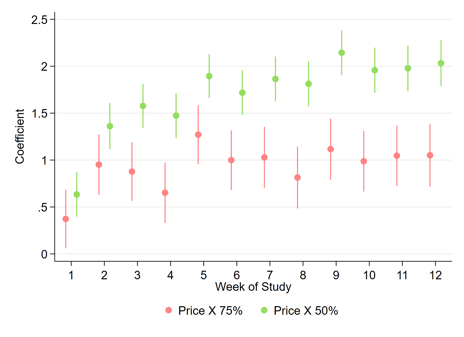
Average Weekly Travel: All Groups
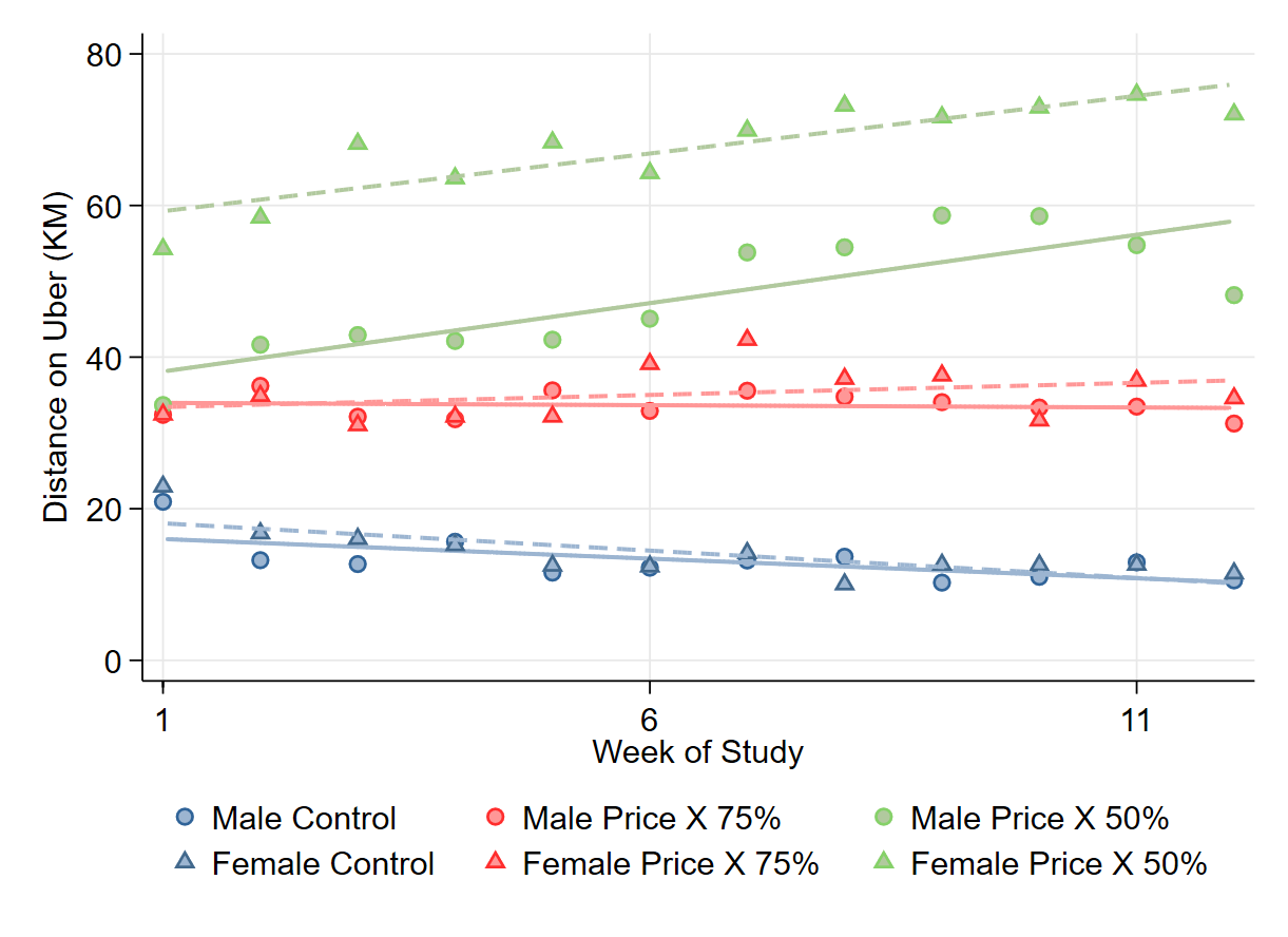
Appendix A: Experimental Design
Experimental Design Appendix A
A1. Price Information for Treated Riders
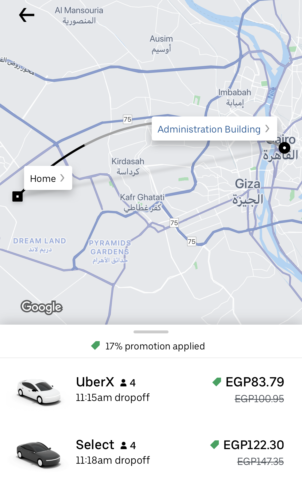
A2. Google Timeline Platform
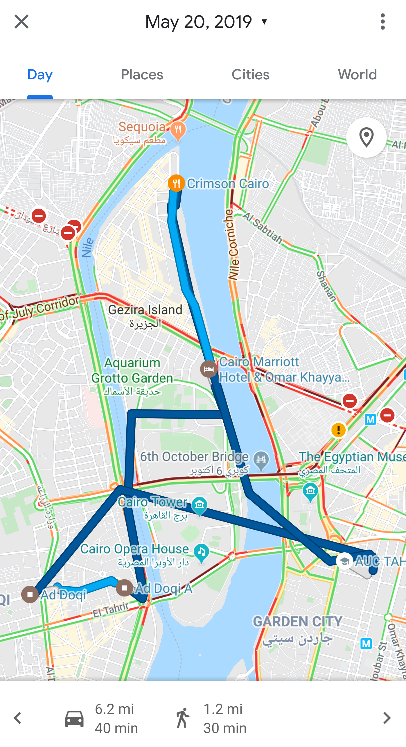
A3. Uber Administrative Data
The figure below illustrates the geographic features (origins/destinations) of the Uber administrative data. The top panel maps a sample of trips for 3 randomly drawn participants in the study. The bottom panel maps the full set of trips for a single randomly drawn day. Trips in the control group are shown in blue, trips in the 25% group are shown in red, and trips in the 50% group are shown in orange.
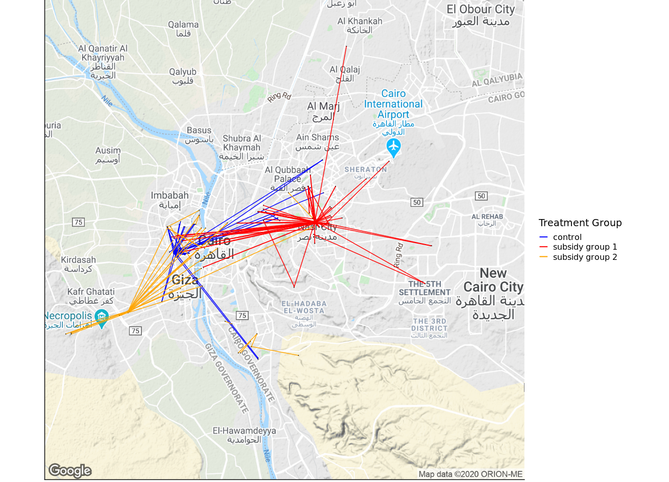
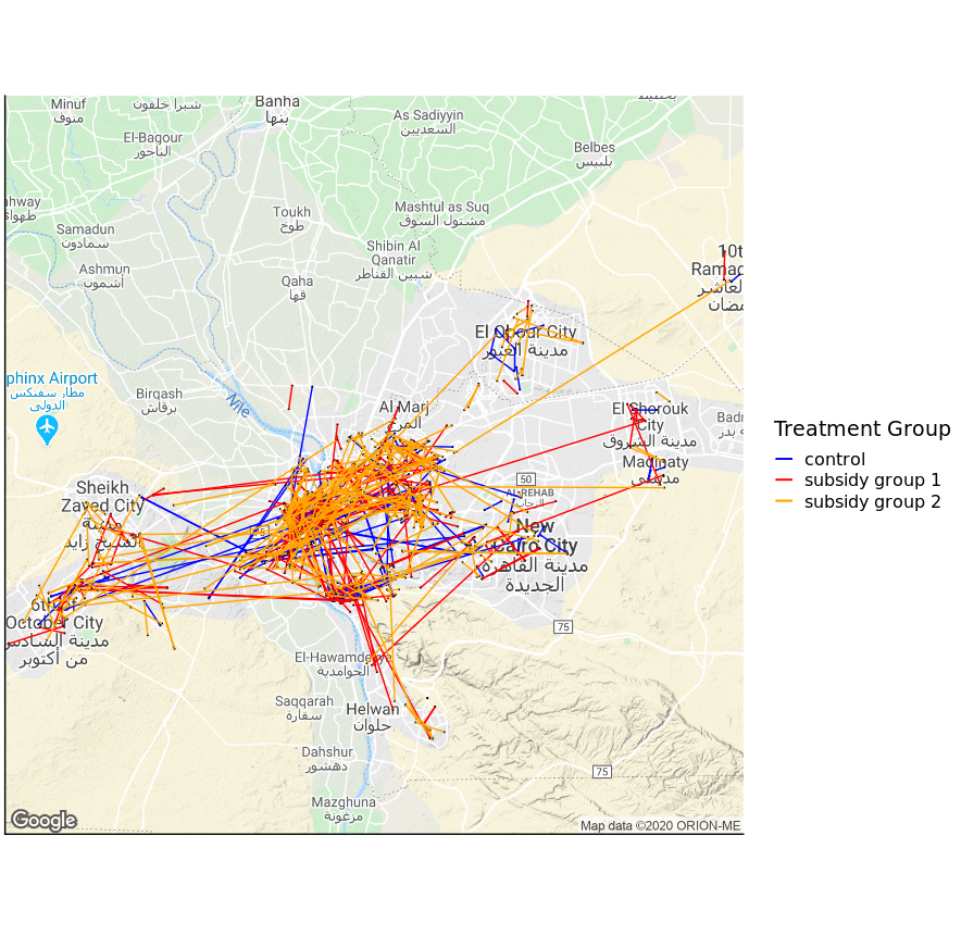
Appendix B: Sample Characteristics, Attrition and Additional Results
Sample Characteristics Appendix B
This appendix includes figures and tables that provide additional detail and insights from the experiment. The first two figures describe baseline travel behavior and beliefs, split by gender. Table B.1 reports baseline characteristics and balance tests for baseline covariates. Table B.2 compares baseline characteristics for the sample to a representative sample of the Cairo population. Table B3 shows how budget shares differ by income. Table B.4 provides data on the transportation market in Cairo and 5 other cities in Africa and Latin America, illustrating that the high levels of public transit ridership and female harassment risk on public transit that characterize Cairo are similar in several other large cities in the developing world. Tables B.8-B.9 analyze attrition throughout the study and test for differential response rates by baseline characteristics across treatment groups. Tables B.11 & B.12 estimate Lee bounds for Mobility and Safety.
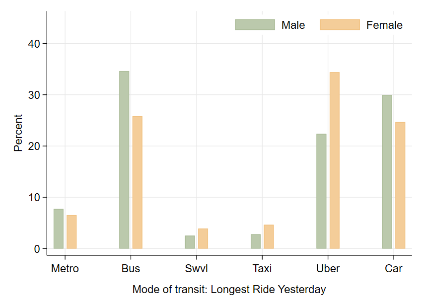
Relative Cost Compared to Uber
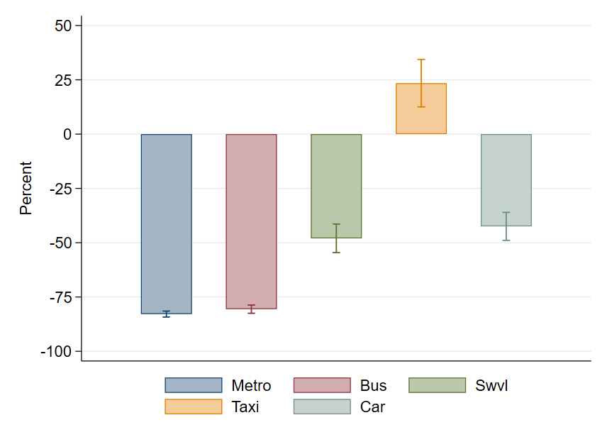
Males
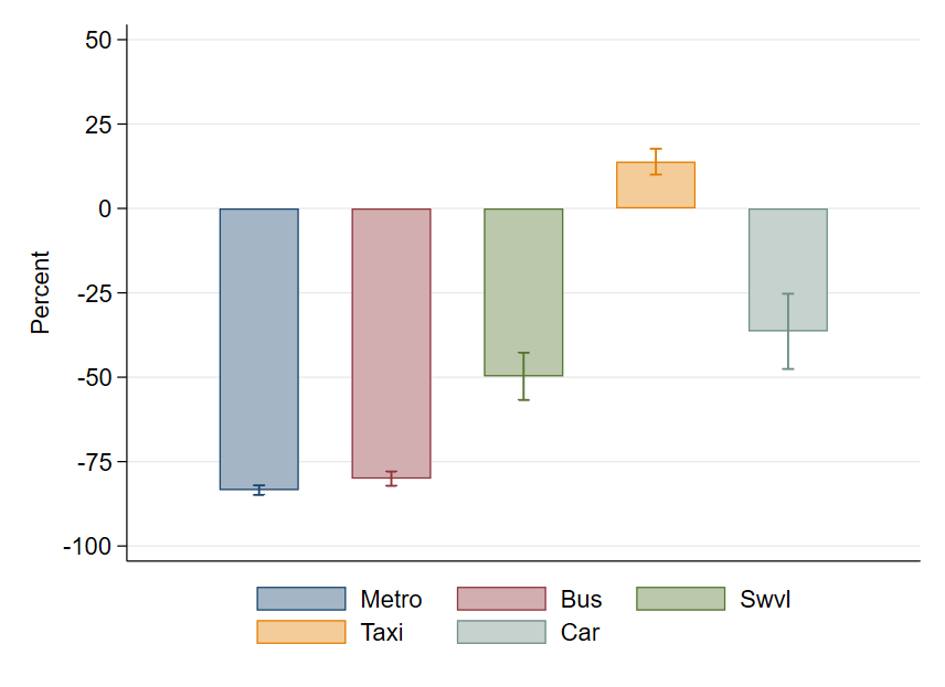
Females
Relative Duration Compared to Uber
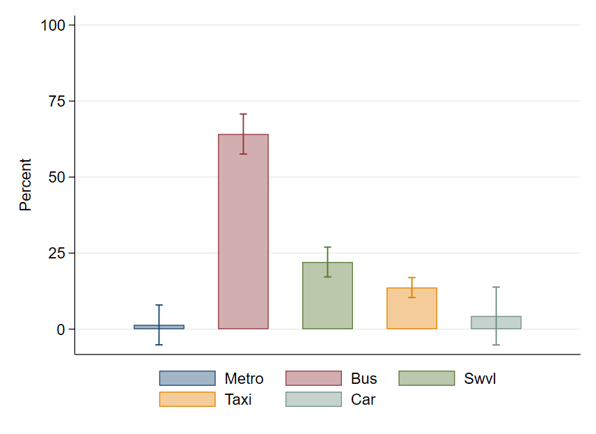
Males
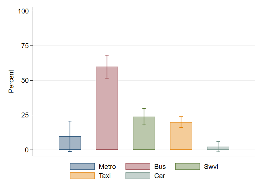
Females
Relative Safety Compared to Uber
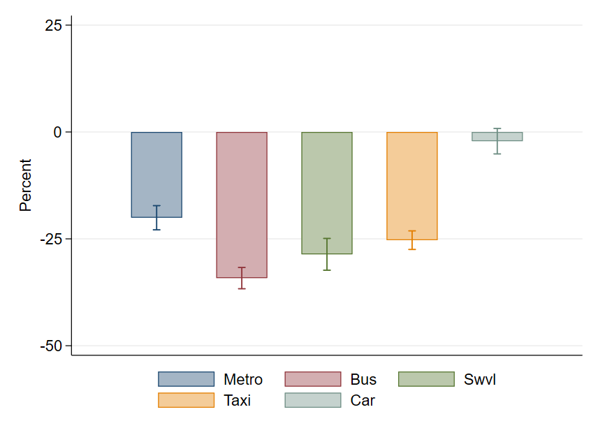
Males
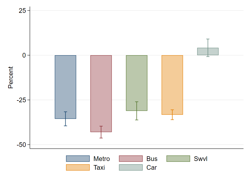
Females
Panel A: Total Weekly Uber Distance (IHS)
25% Price Reduction
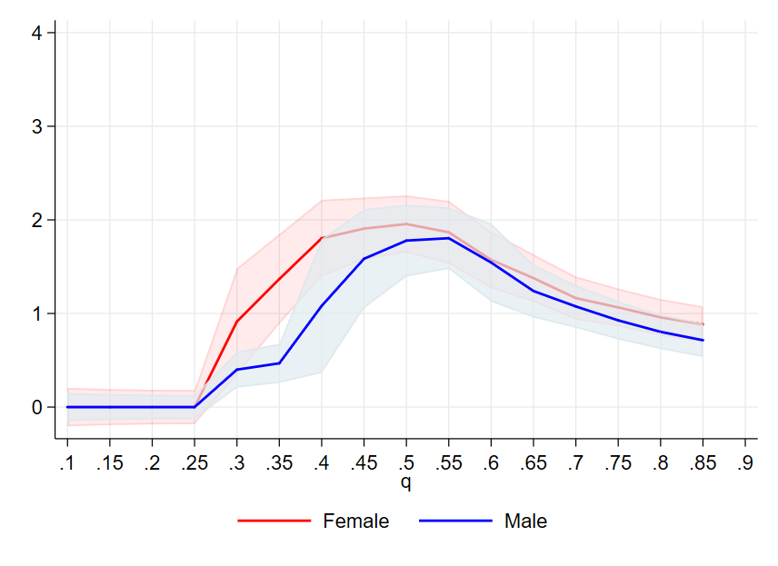
50% Price Reduction
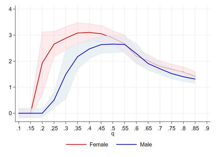
Panel B: Number of Weekly Uber Trips
25% Price Reduction
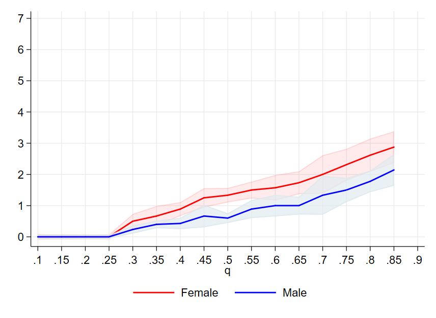
50% Price Reduction
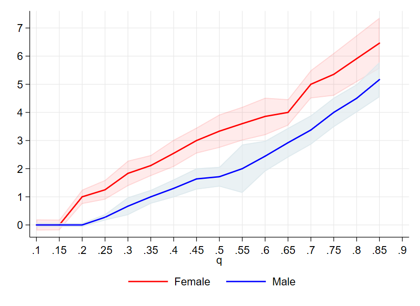
Panel C: Total Distance (IHS)
25% Price Reduction
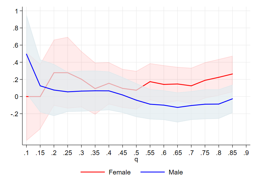
50% Price Reduction
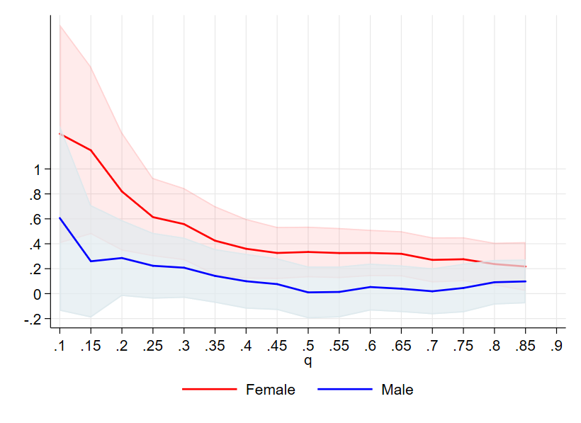
Baseline Characteristics
| Variables | Control | 75% | 50% | 50% vs 75% |
|---|---|---|---|---|
| Mean | vs Control | vs Control | ||
| Female | 0.47 | 0.00 | 0.00 | -0.00 |
| (0.50) | (0.03) | (0.03) | (0.03) | |
| Age | 31.36 | -0.29 | -0.96 | -0.67 |
| (10.65) | (0.72) | (0.80) | (0.77) | |
| Married | 0.50 | -0.00 | -0.06* | -0.05 |
| (0.50) | (0.03) | (0.03) | (0.03) | |
| Monthly Income | 4,655 | -192 | -419 | -226 |
| (6,803) | (430) | (423) | (314) | |
| Currently Working | 0.78 | 0.00 | 0.01 | 0.00 |
| (0.41) | (0.03) | (0.03) | (0.03) | |
| Hours Worked (hours/week) | 44.54 | -0.88 | 0.32 | 1.20 |
| (15.61) | (1.24) | (1.16) | (1.22) | |
| Looking for Work | 0.48 | 0.00 | -0.01 | -0.01 |
| (0.50) | (0.03) | (0.03) | (0.03) | |
| Car Owner | 0.26 | 0.01 | -0.05 | -0.05* |
| (0.44) | (0.03) | (0.03) | (0.03) | |
| Total Weekly Trips | 20.83 | 1.26 | -0.04 | -1.30 |
| (13.66) | (0.90) | (0.88) | (0.86) | |
| Total Mobility (km/week) | 86.33 | -12.59 | -0.66 | 11.93 |
| (200.24) | (11.39) | (12.29) | (9.63) | |
| Total Time in Transit (min/week) | 604.72 | -59.98 | -28.86 | 31.12 |
| (2,698.80) | (144.62) | (146.43) | (87.86) | |
| Velocity (km/hour) | 25.64 | -5.12 | 10.33 | 15.45 |
| (143.54) | (7.65) | (14.24) | (12.77) | |
| Observations | 455 | 954 | 958 | 960 |
| Joint F-test (p-value) | 0.80 | 0.61 | 0.72 |
Notes: Column (1) reports the mean and standard deviation of the control group for a given outcome variable, Column (2) reports the average difference between each variable for those in the Price X 75% treatment group relative to control, Column (3) reports the average difference between each variable for those in the Price X 50% treatment group relative to control, and Column (4) reports the average difference between each variable for those in the Price X 75% treatment group relative to those in the Price X 50% treatment group. The last row in each panel reports the p-value for the F-test from a regression of the treatment dummy on all baseline balance variables. Significance: *.10; **.05; ***.01.
Comparing Experiment Sample to Representative Sample of Cairo
| Overall | Female | Male | ||||
|---|---|---|---|---|---|---|
| (1) | (2) | (3) | (4) | (5) | (6) | |
| Population | Sample | Population | Sample | Population | Sample | |
| Gender | 0.49 | 0.53 | 0 | 0 | 1 | 1 |
| (0.5) | (0.50) | (0.0) | (0.0) | (0.0) | (0.0) | |
| Age | 35.89 | 30.92 | 36.42 | 29.95 | 35.33 | 31.77 |
| (13.81) | (9.54) | (14.11) | (9.89) | (13.47) | (9.15) | |
| Married | 0.60 | 0.49 | 0.63 | 0.45 | 0.57 | 0.52 |
| (0.49) | (0.50) | (0.48) | (0.50) | (0.50) | (0.50) | |
| Hours Worked (hours/week) | 20.67 | 44.47 | 6.76 | 39.05 | 35.20 | 48.15 |
| (26.98) | (16.17) | (16.69) | (28.00) | (17.08) | (16.44) | |
| Currently Working | 0.44 | 0.79 | 0.17 | 0.68 | 0.73 | 0.88 |
| (0.50) | (0.41) | (0.37) | (0.47) | (0.44) | (0.32) | |
| Monthly Income | 1026 | 4403 | 305 | 3434 | 1778 | 5060 |
| (2990) | (5274) | (1415) | (3813) | (3882) | (5987) | |
| College Education | 0.27 | 0.88 | 0.25 | 0.90 | 0.29 | 0.86 |
| (0.44) | (0.32) | (0.43) | (0.30) | (0.45) | (0.34) | |
| High School | 0.33 | 0.09 | 0.29 | 0.08 | 0.35 | 0.10 |
| (0.47) | (0.28) | (0.46) | (0.27) | (0.48) | (0.30) | |
| Less than High School | 0.40 | 0.01 | 0.46 | 0.01 | 0.36 | 0.01 |
| (0.49) | (0.08) | (0.50) | (0.08) | (0.48) | (0.08) | |
| Car Owner | 0.13 | 0.25 | 0.13 | 0.20 | 0.12 | 0.29 |
| (0.33) | (0.43) | (0.34) | (0.40) | (0.32) | (0.46) | |
| Looking for Work | 0.03 | 0.49 | 0.03 | 0.33 | 0.04 | 0.63 |
| (0.18) | (0.50) | (0.17) | (0.47) | (0.19) | (0.48) |
Notes: Columns (1), (3), & (5) report the average values for a representative sample of Cairo residents, taken from the 2018 Egypt Labor Market Panel Survey. Columns (2), (4), & (6) report the values for individuals in our sample. Standard deviations reported in parentheses.
Comparison between Cities
| Cairo | Bogota | Cape Town | Mexico City | Nairobi | Panama City | |
|---|---|---|---|---|---|---|
| % Public Transit | 63% | 60% | 54% | 69% | 60% | 57% |
| Harassment of Women on Public Transit | 86.5% | 80% | 73-90% | 75% | 75% | - |
| Insecurity on Transit | - | 68% | 42% | - | - | 54% |
| % Car Owner | 13% | 15% | 43.8% | 28% | - | 15% |
Notes: These data come from (Ouali et al. (2020); Lombard et al. (2007); Estupi nan et al. (2018); El Deeb (2013); Odhiambo et al. (2021); Ya nez-Pagans et al. (2019)).
Impact of Treatment on Length of Uber Trips
| Total KM per Trip (IHS) | ||
|---|---|---|
| (1) | (2) | |
| Price X 75% | 0.09* | 0.11 |
| (0.05) | (0.08) | |
| Price X 75% * Male | -0.04 | |
| (0.11) | ||
| Price X 50% | 0.17*** | 0.23*** |
| (0.05) | (0.07) | |
| Price X 75% * Male | -0.11 | |
| (0.10) | ||
| Observations | 56802 | 56718 |
| Control Group Mean | 9.0 | 8.9 |
| Control Group Mean (Male) | 9.1 |
Notes: Column (1) reports the impacts of the two treatment arms on the inverse hyperbolic sine of total kilometers traveled in the uber trip. Column (2) reports the results from a specification that interacts treatment with a dummy variable for men. The bottom rows report the control means in levels and split by gender in Column (2). Regressions include strata, cohort and follow-up round fixed effects as well as controls chosen using a double-post-lasso procedure. Standard errors clustered at the individual level in parentheses. Significance: *.10; **.05; ***.01.
Travel on Private vs. Public Transportation
| Total Weekly KM Public (IHS) | Total Weekly KM Private (IHS) | |||
|---|---|---|---|---|
| (1) | (2) | (3) | (4) | |
| Price X 75% | 0.12 | 0.39 | 0.37** | 0.07 |
| (0.19) | (0.26) | (0.18) | (0.25) | |
| Price X 75% * Male | -0.54 | 0.61* | ||
| (0.37) | (0.36) | |||
| Price X 50% | 0.22 | 0.27 | 0.47*** | 0.39 |
| (0.19) | (0.26) | (0.18) | (0.24) | |
| Price X 50% * Male | -0.08 | 0.15 | ||
| (0.37) | (0.36) | |||
| Observations | 3352 | 3352 | 3352 | 3352 |
| Control Group Mean Levels | 74.5 | 38.9 | 127.7 | 106.6 |
| Control Group Mean Levels (Male) | 108.0 | 147.7 |
Notes: Notes: Column (1) reports the impacts of the two treatment arms on the inverse hyperbolic sine of total kilometers on public transportation (bus & metro). Column (2) reports the results from a specification that interacts treatment with a dummy variable for men. The bottom rows report the control means in levels and split by gender in Column (2). Columns (3) & (4) report impacts on on private travel (i.e. taxi, Uber, and private car). Regressions include strata, cohort and follow-up round fixed effects as well as controls chosen using a double-post-lasso procedure. Standard errors clustered at the individual level in parentheses. Significance: *.10; **.05; ***.01.
Impacts of Treatment on Trip Purpose
| Work | School | Leisure | Other | |||||
|---|---|---|---|---|---|---|---|---|
| (1) | (2) | (3) | (4) | (5) | (6) | (7) | (8) | |
| Price X 75% | 0.00 | -0.03 | 0.01 | 0.00 | -0.02 | 0.01 | 0.02 | 0.01 |
| (0.05) | (0.04) | (0.02) | (0.02) | (0.05) | (0.04) | (0.01) | (0.01) | |
| Price X 75% * Male | -0.05 | -0.02 | 0.08 | -0.01 | ||||
| (0.08) | (0.03) | (0.08) | (0.02) | |||||
| Price X 50% | -0.05 | -0.04 | 0.03 | 0.01 | 0.01 | 0.02 | 0.02 | 0.00 |
| (0.05) | (0.04) | (0.02) | (0.02) | (0.05) | (0.04) | (0.01) | (0.01) | |
| Price X 50% * Male | 0.03 | -0.04 | 0.04 | -0.03 | ||||
| (0.07) | (0.03) | (0.07) | (0.02) | |||||
| Observations | 1661 | 1661 | 1661 | 1661 | 1661 | 1661 | 1661 | 1661 |
| Control Group Mean Levels | 0.47 | 0.39 | 0.06 | 0.09 | 0.46 | 0.51 | 0.01 | 0.01 |
| Control Group Mean Levels (Male) | 0.54 | 0.03 | 0.43 | 0.01 |
Notes: Table reports the coefficients from 4 discrete regressions of each purpose on a binary outcome that takes the value 1 if the individual reported taking that purpose of transportation for their longest trip the day of our follow-up survey. Even numbered columns report the results from a specification that interacts treatment with a dummy variable for men. “Leisure" category includes trips with the following purposes: personal, family visit, friend visit, shopping and health. Standard errors clustered at the individual level in parentheses. Significance: *.10; **.05; ***.01.
Response Rates
| (1) | (2) | (3) | (4) | (5) | |
|---|---|---|---|---|---|
| Any Follow-Up | Follow-Up 1 | Follow-Up 2 | Follow-Up 3 | Follow-Up 4 | |
| Price X 75% | 0.02 | -0.01 | 0.05* | 0.04 | 0.02 |
| (0.01) | (0.03) | (0.03) | (0.03) | (0.03) | |
| Price X 50% | 0.03** | 0.02 | 0.08*** | 0.06* | 0.08** |
| (0.01) | (0.02) | (0.03) | (0.03) | (0.03) | |
| Control Group Response Rate | 0.94*** | 0.82*** | 0.78*** | 0.40*** | 0.38*** |
| (0.01) | (0.02) | (0.02) | (0.02) | (0.02) | |
| Observations | 1373 | 1373 | 1373 | 1373 | 1373 |
Notes: Columns (1) reports the coefficients from a regression on a binary outcome that takes the value 1 if the individual reported to answer any follow-up survey and 0 otherwise. Columns (2), (3), (4), & (5) report the result for each follow-up. Standard errors clustered at the individual level in parentheses. Significance: *.10; **.05; ***.01.
Impacts of Observable Characteristics on Response Rates (All Follow-Ups)
| Dependent variable: Response to Follow-Up | ||
|---|---|---|
| (1) | (2) | |
| Price X 75% | Price X 50% | |
| treatment | -0.09 | -0.13 |
| (0.11) | (0.11) | |
| Car | -0.06** | -0.06** |
| (0.03) | (0.03) | |
| Education | -0.02 | -0.02 |
| (0.02) | (0.02) | |
| Married | -0.02 | -0.02 |
| (0.02) | (0.02) | |
| Female | 0.09*** | 0.09*** |
| (0.02) | (0.02) | |
| Looking for work | 0.00 | 0.00 |
| (0.00) | (0.00) | |
| Total distance | 0.00 | -0.00 |
| (0.00) | (0.00) | |
| Treatment * Car | 0.03 | 0.08** |
| (0.04) | (0.04) | |
| Treatment * Education | 0.03 | 0.03 |
| (0.02) | (0.02) | |
| Treatment * Married | -0.01 | -0.02 |
| (0.03) | (0.03) | |
| Treatment * Female | -0.04 | 0.03 |
| (0.03) | (0.03) | |
| Treatment * Looking for work | 0.00 | 0.00 |
| (0.00) | (0.00) | |
| Treatment * Total distance | 0.00 | 0.00 |
| (0.00) | (0.00) | |
| Constant | 0.67*** | 0.67*** |
| (0.08) | (0.08) | |
| Observations | 3632 | 3644 |
| F-Test | 0.71 | 1.30 |
| (P Value) | (0.64) | (0.25) |
Notes: Columns (1) reports the coefficients from a regression on a binary outcome that takes the value 1 if the individual reported to answer any follow-up survey and 0 otherwise given the 25% treatment group, some control variables and the interaction of the treatment with the controls. Column (2) reports the same estimation for the 50% treatment group. The F-Test shows joint significance for the control variables when interacted with the treatments. Standard errors clustered at the individual level in parentheses. Significance: *.10; **.05; ***.01.
Impacts of Observable Characteristics on Response Rates (1 Follow-Up Min.)
| Dependent variable: Response to Follow-Up | ||
|---|---|---|
| (1) | (2) | |
| Price X 75% | Price X 50% | |
| Treatment | -0.01 | -0.13 |
| (0.10) | (0.09) | |
| Car | -0.04* | -0.04** |
| (0.02) | (0.02) | |
| Education | -0.01 | -0.01 |
| (0.01) | (0.01) | |
| Married | -0.01 | -0.01 |
| (0.02) | (0.02) | |
| Female | 0.00 | 0.00 |
| (0.02) | (0.02) | |
| Looking for work | 0.00 | 0.00 |
| (0.00) | (0.00) | |
| Distance | 0.00 | 0.00 |
| (0.00) | (0.00) | |
| Treatment * Car | 0.03 | 0.04 |
| (0.03) | (0.03) | |
| Treatment * Education | 0.01 | 0.03* |
| (0.02) | (0.02) | |
| Treatment * Married | 0.00 | -0.02 |
| (0.03) | (0.03) | |
| Treatment * Female | -0.03 | 0.01 |
| (0.03) | (0.03) | |
| Treatment * Look For Work | 0.00 | 0.00 |
| (0.00) | (0.00) | |
| Treatment * Total Distance | 0.00** | 0.00 |
| (0.00) | (0.00) | |
| Constant | 1.01*** | 1.01*** |
| (0.07) | (0.06) | |
| Observations | 908 | 911 |
| F-Test | 1.17 | 0.91 |
| (P Value) | (0.32) | (0.49) |
Notes: Columns (1) reports the coefficients from a regression on a binary outcome that takes the value 1 if the individual reported to answer at least 1 follow-up survey and 0 otherwise given the 25% treatment group, some control variables and the interaction of the treatment with the controls. Column (2) reports the same estimation for the 50% treatment group. The F-Test shows joint significance for the control variables when interacted with the treatments. Standard errors clustered at the individual level in parentheses. Significance: *.10; **.05; ***.01.
Lee Bounds for Total Mobility
| Overall | Female | Male | |||||||
|---|---|---|---|---|---|---|---|---|---|
| (1) | (2) | (3) | (4) | (5) | (6) | (7) | (8) | (9) | |
| Lower | Higher | Main Estimate | Lower | Higher | Main Estimate | Lower | Higher | Main Estimate | |
| Price X 75% | -0.01 | 0.5*** | 0.1 | 0.11 | 0.65*** | 0.18 | -0.11 | 0.38*** | 0.03 |
| (0.00) | (0.08) | (0.09) | (0.14) | (0.12) | (0.14) | (0.12) | (0.10) | (0.12) | |
| Price X 50% | 0.11 | 0.74*** | 0.35*** | 0.24* | 0.90*** | 0.49*** | 0.02 | 0.58*** | 0.23** |
| (0.08) | (0.07) | (0.08) | (0.12) | (0.11) | (0.12) | (0.11) | (0.10) | (0.11) |
Notes: Columns (1), (4) & (7) report the lower Lee bounds from regressions of total mobility on treatment. To generate the lower Lee bounds we compare the proportion in treatment and control groups who respond to the surveys and trim the excess respondents with the highest values in the group with more respondents. For columns (2), (5) & (8) we repeat this process but remove the lowest values. In columns (3), (6), & (9) we reproduce the main results. Standard errors clustered at the individual level in parentheses. Significance: *.10; **.05; ***.01.
Lee Bounds for Safety
| Overall | Female | Male | |||||||
|---|---|---|---|---|---|---|---|---|---|
| (1) | (2) | (3) | (4) | (5) | (6) | (7) | (8) | (9) | |
| Lower | Higher | Main Estimate | Lower | Higher | Main Estimate | Lower | Higher | Main Estimate | |
| Price X 75% | -0.71*** | 0.39*** | 0.06 | -0.62*** | 0.31*** | 0.19*** | -0.78*** | 0.32*** | 0.05 |
| (0.06) | (0.05) | (0.06) | (0.10) | (0.09) | (0.10) | (0.08) | (0.06) | (0.08) | |
| Price X 50% | -0.77*** | 0.44*** | 0.09* | -0.69*** | 0.76*** | 0.22*** | -0.85*** | 0.33*** | 0.01 |
| (0.06) | (0.05) | (0.06) | (0.10) | (0.07) | (0.09) | (0.08) | (0.06) | (0.08) |
Notes: Columns (1), (4) & (7) report the lower Lee bounds from regressions of total mobility on treatment. To generate the lower Lee bounds we compare the proportion in treatment and control groups who respond to the surveys and trim the excess respondents with the highest values in the group with more respondents. For columns (2), (5) & (8) we repeat this process but remove the lowest values. In columns (3), (6), & (9) we reproduce the main results. Standard errors clustered at the individual level in parentheses. Significance: *.10; **.05; ***.01.
Appendix C: Measuring Mobility
Measuring Mobility Appendix C
This appendix provides additional detail on the measurement of mobility across the three data sources used in the study: (1) Uber administrative data on trips, (2) trip surveys, and (3) total travel using Google Timeline.
Measuring Total Travel with Google Timeline
In this section, we evaluate the consistency of measurements across different data sources and report results from a set of validation exercises that evaluated differences in distance measurements between a manually constructed daily travel log, Uber administrative data, and Google Timeline data prior to the study.
Google Timeline Validation
Over a 5-day period prior to the study, we conducted a validation exercise to evaluate measurement error in Google Timeline data. As depicted in Figure C.1, we created a manual trip log that records the distances of travel taken by Uber and private car. We then compared the distances recorded in the log to the distance measurements collected on the Uber platform and in our Google Timeline.

Table C.1 reports the results from the validation exercise, which indicates that Timeline understates total travel by about 12.5% relative to the manual log. In our analysis, we report our results in percentage terms using an IHS transformation and restrict all comparisons between data sources to comparisons of percentage effects, further helping to correct for any uniform underestimate of overall distance measured on Google Timeline. The difference is 12.6% when taking an Uber trip and by 12% when not taking an Uber trip, providing some evidence that GPS functionality when an individual is taking an Uber trip does not result in differences in Timeline measurements of total travel. When we compare data from Uber’s administrative data to manual logs, we find that the administrative data understates total travel by 2.9%. This is likely because Uber’s log utilizes data from an application on the driver’s phone, which is built to collect more accurate data (but is much more battery intensive).
Comparison of Manual Travel Log, Google Timeline, Uber Admin
| Category | # of trips | Log Distance | Uber Distance | Timeline Distance | Log-Timeline (%) | Log-Uber (%) |
|---|---|---|---|---|---|---|
| Uber Trips | 11 | 169.30 | 174.20 | 147.90 | 12.62% | 2.89% |
| Non-Uber Trips | 3 | 33.70 | - | 29.70 | 11.94% | - |
| All Vehicle Trips | 14 | 202.90 | - | 177.60 | 12.51% | - |
Notes: All distances are reported in kilometers.
GPS tracking on Uber vs. Non-Uber Trips
The validation exercise above suggests that measurement error in Google Timeline measurements is similar across Uber and non-Uber trips. It is possible that participants disable their GPS while using modes other than Uber. While this would require that a participant fully disables navigation services during travel, participants may do this in certain cases to preserve battery life. A benefit of the Timeline app is that it is optimized for battery life, potentially reducing participant concerns about battery use. Either of these issues could bias our experimental results if they differentially affect the measurement of total travel for the treated group (who use Uber more).
Using data from the baseline survey, Table C.2 reports the results of a regression of total travel on the number of trips taken using each mode for the same period. While disentangling mode-specific measurement error from mode-specific differences in trip lengths would require independent measurements of distances traveled in each of the recorded trips, these correlations do not suggest that Uber trips have an outsized influence in the total distance measurement. \\
Previous Day Km on Trips (Baseline)
| (1) | |
|---|---|
| Total KM Previous Day (IHS) | |
| Metro Trips | 0.21*** |
| (0.06) | |
| Bus Trips | 0.23*** |
| (0.03) | |
| Taxi Trips | 0.17** |
| (0.07) | |
| Uber Trips | 0.31*** |
| (0.05) | |
| Car Trips | 0.27*** |
| (0.03) | |
| Observations | 1373 |
Notes: This table reports the coefficients from a regression of previous day kilometers on the number of trips taken that day. Standard errors clustered at the individual level in parentheses. Significance: *.10; **.05; ***.01.
We then compare the coefficient of variation in total distance traveled on days that include Uber trips and those that do not. If the use of Uber makes Google Timeline more precise, then we would expect less variation in the data collected on days when Uber trips are taken. Directly comparing the variance would not be appropriate because as distance traveled increases, the overall variance will also increase. For this reason, we utilize the coefficient of variation (the standard deviation divided by the mean), which provides a scale invariant measure. Table C.3 reports the results of this analysis. We find that the coefficient of variation are very similar on days with and without an Uber, suggesting that this potential bias is not a first-order concern for our analysis.
Coefficient of Variation
| Overall | Control | Subsidy 25% | Subsidy 50% | |
|---|---|---|---|---|
| (1) | (2) | (3) | (4) | |
| Day With Uber | 1.41 | 1.32 | 1.47 | 1.44 |
| [1.19, 1.47] | [1.12, 1.36] | [1.27, 1.68] | [1.24, 1.68] | |
| Day Without Uber | 1.52 | 1.42 | 1.55 | 1.59 |
| [1.23,1.59] | [1.33,1.80] | [1.36, 1.70] | [1.53, 1.95] |
Notes: This table reports the coefficient of variation of distance reported on Google Timeline separated by days in which an individual took an Uber ride and days in which they did not take an Uber ride. 95% confidence intervals reported in brackets.
Uber Travel (Administrative Data) vs Total Travel (Timeline)
Next, we examine the robustness of our results by utilizing Uber’s administrative data to identify instances of measurement error in the Google Timeline. Figure C.2 plots the total distance traveled from a participant’s Timeline against the distance recorded on Uber over the same period. During the average 3-day period with no Uber travel, a participant’s total travel is 77 km. For each additional 1 km of Uber travel, the total travel increases by 0.26 km on average. Table B.10 reports these estimates by treatment group. We do not find any evidence of systematic differences in the relationships between Uber and Timeline measurements across the groups. \\
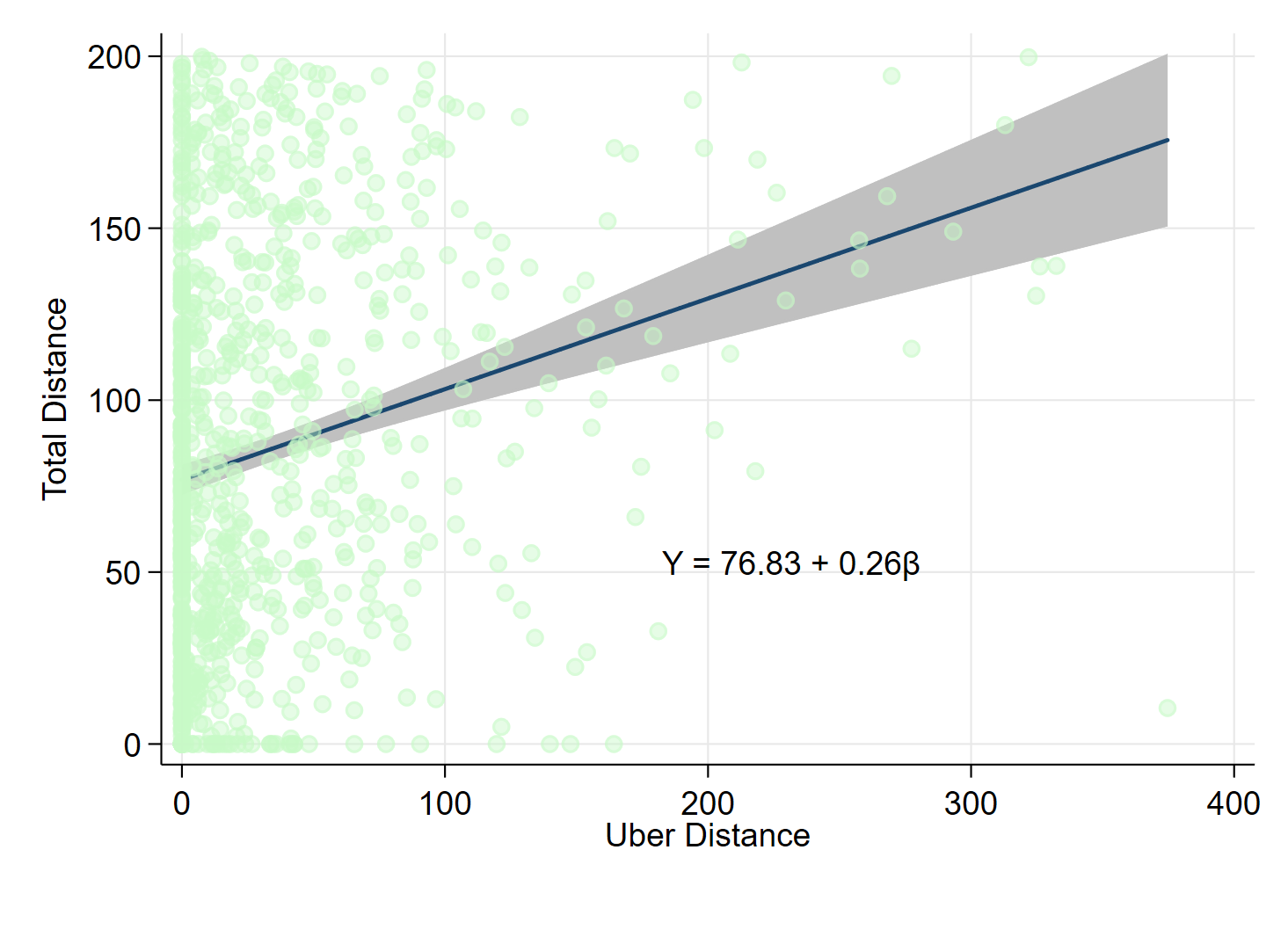
Total Distance vs Uber Distance Regression
| Overall | Control | Subsidy 25% | Subsidy 50% | |
|---|---|---|---|---|
| (1) | (2) | (3) | (4) | |
| Beta Estimator | 0.27*** | 0.24* | 0.20** | 0.29*** |
| (0.04) | (0.14) | (0.07) | (0.05) |
Notes: Column (1) reports the beta estimator of the regression of Total distance on Uber distance for the same period. Columns (2), (3) & (4) report the beta estimators of the regression of Total distance on Uber distance by treatment group. Standard errors in parentheses. Significance: *.10; **.05; ***.01.
Since a participant’s Uber travel should be captured in their total daily distance, we expect to see that $Total Distance > Uber Distance$. In Table C.5, we identify observations where the measurement of Uber travel exceeds the measurement of total travel, which indicates measurement error that could occur during intervals when a GPS is not collecting data or battery failure. This occurs in 13.6% of the observations in the sample.
Total Travel (Timeline) vs Uber Travel (Administrative Data)
| 3 Days | Distance Fraction | Average Total Distance (km) | |
|---|---|---|---|
| Total Distance \geq Uber distance | 86.37% | 98.25 | |
| Uber distance \geq Total Distance | 13.63% | 68.57 |
To examine the effects of these observations on our results on the effects of price reductions on total mobility, we produce a version of Table 2 that omits the 13.6% of observations where Uber travel exceeds total travel. We view this set of inconsistent observations as instances of likely under-reporting of total travel by Google Timeline. We find that removing these observations slightly increases our estimates of effects of treatment on total mobility, likely due to the fact that these observations fall at the low end of the distribution of observations of total travel, at the upper end of the distribution of observations of Uber travel (which are more likely to be found in the treatment groups). However, the estimates are not different from estimates produced with the full sample. Whereas the point estimate for the effect of a 50% price reduction was 0.40 IHS points in Table 2, the effects in this restricted sample are 0.53 IHS points.
Impacts in Total Mobility (Sample: $Total Distance > Uber Distance$)
| Total KM Past Week (IHS) | ||
|---|---|---|
| (1) | (2) | |
| Price X 75% | 0.13 | 0.22 |
| (0.11) | (0.18) | |
| Price X 75% * Male | -0.19 | |
| (0.23) | ||
| Price X 50% | 0.53*** | 0.67*** |
| (0.10) | (0.15) | |
| Price X 50% * Male | -0.27 | |
| (0.20) | ||
| Observations | 3073 | 3071 |
| Control Group Mean | 212.95 | 151.16 |
| Control Group Mean (Male) | 267.29 |
Notes: Table reports estimates from Table 2, restricting the sample to observations where $Total Distance > Uber Distance$. Column (1) reports the impacts of the two treatment arms on the inverse hyperbolic sine of total kilometers traveled in the three days prior to our follow-up survey as reported by Google Maps’ “Timeline" feature. Column (2) reports the results from a specification that interacts treatment with a dummy variable for men. The bottom rows of report the control means in levels and split by gender in Column (2). Regressions include strata, cohort and follow-up round fixed effects as well as controls chosen using a double-post-lasso procedure. Standard errors clustered at the individual level in parentheses. Significance: *.10; **.05; ***.01.
Mode Choice
We measure mode choice using two different survey questions: (1) total number of trips taken on each mode on the day before the survey, and (2) mode used for the longest trip (in distance) on the day before the survey. Table C.7 reports treatment effects across the two measures. Panel A reports effects on the mode share for all trips while Panel B reports effects on the mode share for longest trips. We find that these two measures are highly consistent, indicating that treatment effects on mode substitution on longest trips are reflective of overall effects.
Travel Mode Choice
| Panel A: Longest Trip | ||||||||||
|---|---|---|---|---|---|---|---|---|---|---|
| Metro | Bus | Taxi | Uber/Careem | Car | ||||||
| (1) | (2) | (3) | (4) | (5) | (6) | (7) | (8) | (9) | (10) | |
| Price X 75% | 0.00 | -0.02 | -0.03 | -0.05 | -0.02** | -0.03** | 0.07*** | 0.09*** | -0.02 | 0.01 |
| (0.01) | (0.02) | (0.02) | (0.04) | (0.01) | (0.01) | (0.02) | (0.03) | (0.02) | (0.03) | |
| Price X 75% * Male | 0.03 | 0.02 | 0.02 | -0.04 | -0.04 | |||||
| (0.03) | (0.05) | (0.01) | (0.04) | (0.05) | ||||||
| Price X 50% | 0.00 | -0.01 | -0.09*** | -0.11*** | -0.02** | -0.03** | 0.11*** | 0.12*** | 0.00 | 0.03 |
| (0.01) | (0.02) | (0.02) | (0.03) | (0.01) | (0.01) | (0.02) | (0.03) | (0.02) | (0.03) | |
| Price X 50% * Male | 0.02 | 0.03 | 0.02 | -0.02 | -0.06 | |||||
| (0.03) | (0.05) | (0.01) | (0.04) | (0.05) | ||||||
| Observations | 3186 | 3186 | 3186 | 3186 | 3186 | 3186 | 3186 | 3186 | 3186 | 3186 |
| Control Group Mean | 0.06 | 0.06 | 0.33 | 0.36 | 0.03 | 0.02 | 0.21 | 0.16 | 0.32 | 0.34 |
| Control Group Mean (Male) | 0.07 | 0.29 | 0.04 | 0.26 | 0.29 |
| Panel B: Proportion of Trips | ||||||||||
|---|---|---|---|---|---|---|---|---|---|---|
| Metro | Bus | Taxi | Uber/Careem | Car | ||||||
| (1) | (2) | (3) | (4) | (5) | (6) | (7) | (8) | (9) | (10) | |
| Price X 75% | -0.00 | -0.02 | -0.03 | -0.04 | -0.01 | -0.02* | 0.06*** | 0.06* | -0.02 | 0.01 |
| (0.01) | (0.01) | (0.02) | (0.03) | (0.01) | (0.01) | (0.02) | (0.03) | (0.02) | (0.03) | |
| Price X 75% * Male | 0.02 | 0.02 | 0.02 | -0.00 | -0.04 | |||||
| (0.02) | (0.04) | (0.01) | (0.04) | (0.04) | ||||||
| Price X 50% | 0.00 | 0.00 | -0.10*** | -0.11*** | -0.02** | -0.02* | 0.12*** | 0.12*** | -0.01 | 0.00 |
| (0.01) | (0.02) | (0.02) | (0.03) | (0.01) | (0.01) | (0.02) | (0.03) | (0.02) | (0.03) | |
| Price X 50% * Male | 0.00 | 0.02 | 0.01 | -0.01 | -0.01 | |||||
| (0.02) | (0.04) | (0.01) | (0.04) | (0.04) | ||||||
| Observations | 3133 | 3133 | 3133 | 3133 | 3133 | 3133 | 3133 | 3133 | 3133 | 3133 |
| Control Group Mean | 0.06 | 0.06 | 0.34 | 0.29 | 0.04 | 0.05 | 0.24 | 0.29 | 0.32 | 0.31 |
| Control Group Mean (Male) | 0.06 | 0.39 | 0.03 | 0.19 | 0.33 |
Notes: Panel A reports the coefficients from 5 discrete regressions of each mode on a binary outcome that takes the value 1 if the individual reported taking that mode of transportation for their longest trip the day our follow-up survey. Even numbered columns report the results from a specification that interacts treatment with a dummy variable for men. The bottom rows report the control means in levels, split by gender in even numbered columns. Panel B reports the coefficients from 5 regressions on the proportion of trips taken the previous day of our follow-up survey. Even numbered columns report the results from a specification that interacts treatment with a dummy variable for men. The bottom rows report the control means in levels, split by gender in even numbered columns. Regressions include strata, cohort and follow-up round fixed effects as well as controls chosen using a double-post-lasso procedure. Standard errors clustered at the individual level in parentheses. Significance: *.10; **.05; ***.01.
Robustness: Time Spent on Different Modes
Figure C.3 plots histograms of the fraction of time spent on a participants’ longest trip (self-reported) relative to time recorded in travel by Google Timeline. We note that on 14% of trips, participants report spending more time on their longest trip than the total recorded travel. This does not vary by treatment group -- Control Group: 13.58%; 25% Treatment Group: 15.44%; 50% Treatment Group: 13.21%. We split the sample using this histogram into two groups: (1) participant-days where the longest trip is a large fraction of total travel and (2) participant-days where the longest trip is a small fraction of total travel.
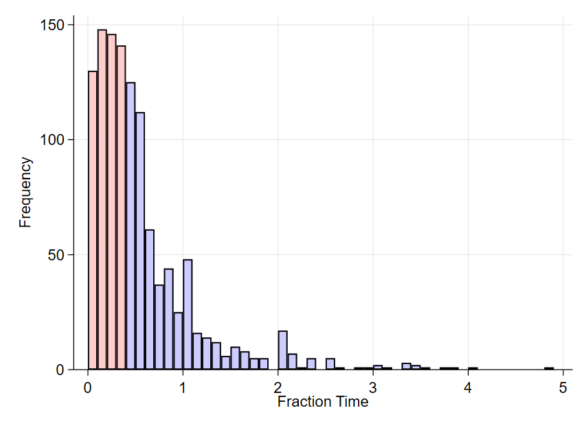
Control Group
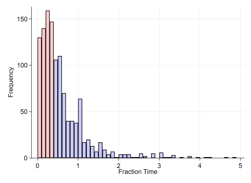
Subsidy 25%
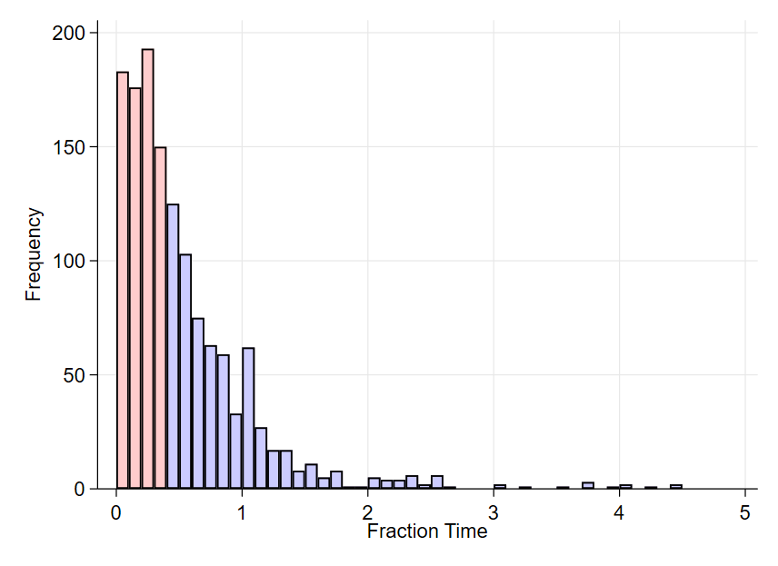
Subsidy 50%
Velocity
Figure C.4 describes the average speed of all movements (km/hour) recorded on participant mobile devices using measurements of distance and time spent traveling. On average velocities range from 20-26 km/hour.
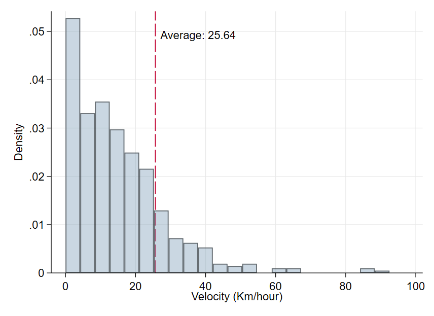
Control Group
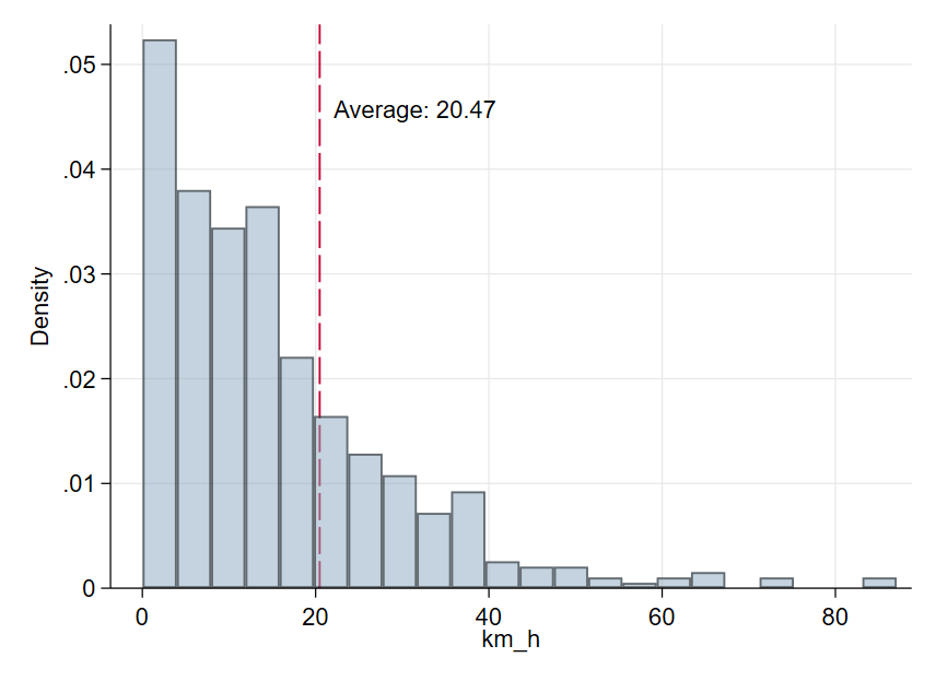
Subsidy 25%
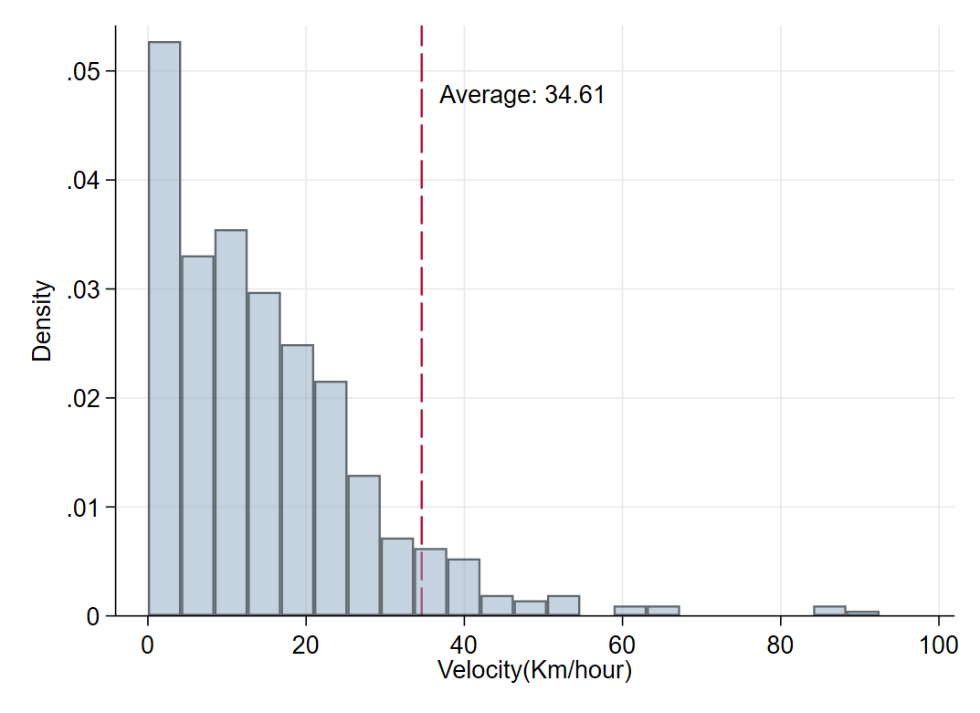
Subsidy 50%
Appendix D: Multiple Hypothesis Testing
Multiple Hypothesis Testing Appendix D
This appendix replicates all of the regressions from the main tables after adjusting for multiple hypotehsis testing concerns using strategies outlined in (List et al. (2019); List et al. (2021)). To maximize power we implement a regression where we pool the treatments into one variable that is equal to 0.75 in the case of a 25% subsidy, and 0.5 in the case of a 50% subsidy.
MHT for Table 1. Impacts of Uber Subsidies on Uber Utilization
| Weekly KM on Uber (IHS) | Weekly Trips on Uber | |||
|---|---|---|---|---|
| (1) | (2) | (3) | (4) | |
| Subsidy | 3.4*** | 3.7*** | 7.32*** | 8.24*** |
| (0.16) | (0.23) | (0.40) | (0.21) | |
| Subsidy * Male | -0.54* | -1.68* | ||
| (0.32) | (0.62) | |||
| Observations | 16440 | 16440 | 16440 | 16440 |
| Control Group Mean Levels | 13.6 | 14.1 | 1.5 | 1.6 |
| Control Group Mean Levels (Male) | 13.2 | 1.5 |
Notes: Column (1) reports the impacts of the continuous treatment on the inverse hyperbolic sine of weekly kilometers traveled on Uber. Column (2) reports the results from a specification that interacts a dummy variable for men, showcasing the differential impact the treatment has for that subgroup. Columns (3) & (4) report the estimates from a regression on the weekly number of trips taken on Uber (in levels). P-values are adjusted to address multiple hypothesis testing concerns following (List et al. (2019)) & (List et al. (2021)). Significance with adjusted p-values, p<0.1*, 0.05**, 0.01***..
MHT for Table 2. Experiments on the Length and Salience of the Price Reduction
| Long Experiment 1st Week | Preannounced Short Experiment | Unannounced Short Experiment | ||||
|---|---|---|---|---|---|---|
| (1) | (2) | (3) | (4) | (5) | (6) | |
| Weekly KM | Trips | Weekly KM | Trips | Weekly KM | Trips | |
| Subsidy | 1.32*** | 4.23*** | 4.14* | 3.78 | 1.34*** | 2.75*** |
| (0.347) | (0.783) | (1.87) | (2.37) | (0.36) | (0.71) | |
| Subsidy * Male | -0.165 | -1.57 | -2.4 | -2.1 | 0.4 | 1.95 |
| (0.479) | (0.94) | (2.52) | (3.29) | (0.52) | (1.11) | |
| Observations | 1370 | 1370 | 1000 | 1000 | 1500 | 1500 |
| Control Mean (Levels) | 22.9 | 2.6 | 13.4 | 2.0 | 20.4 | 2.2 |
| Control Mean for Men | 20.9 | 2.2 | 18.7 | 2.2 | 21.4 | 2.1 |
Notes: Columns (1), (3), & (5) report the impacts of the continuous treatment and their interactions with a male dummy variable, on the inverse hyperbolic sine of weekly kilometers traveled on Uber during the first week of the experiment, the pre-announced experiment and the unannounced experiment respectively.Columns (2), (4), & (6) report the same but with number of trips as the outcome variable. P-values are adjusted to address multiple hypothesis testing concerns following (List et al. (2019)) & (List et al. (2021)). Significance with adjusted p-values, p<0.1*, 0.05**, 0.01***.
MHT for Table 3. Trips to University, Hospital and Metro
| Unique Location Visited | University Trips | Hospital Trips | Metro Trips | |||||
|---|---|---|---|---|---|---|---|---|
| (1) | (2) | (3) | (4) | (5) | (6) | (7) | (8) | |
| Subsidy | 28.28*** | 42.63** | 34.39*** | 47.13*** | 23.59** | 27.13*** | ||
| (6.34) | (12.47) | (6.54) | (10.06) | (3.65) | (6.057) | |||
| Subsidy * Male | -24.16 | -20.03 | -6.36 | |||||
| (13.75) | (13.39) | (7.45) | ||||||
| Observations | 1404 | 1404 | 16452 | 16452 | 16452 | 16452 | 16452 | 16452 |
| Control Group Mean Levels | 8.9 | 8.8 | 5.3 | 5.6 | 7.2 | 6.1 | 4.7 | 4.8 |
| Control Group Mean Levels (Male) | 8.9 | 5.0 | 8.1 | 4.7 |
Notes: Column (1) reports the impacts of the continuous treatment on the unique weekly number of grids visited in the start and finish locations
on Uber trips. Columns (3), (5), & (7) report the impacts on the weekly number of trips that started or end close to an university, hospital and metro station (multiplied by 100 to make coefficients easier to read). Columns (2), (4), (6), & (8) do the same but include an interaction term for men. P-values are adjusted to address multiple hypothesis testing concerns following (List et al. (2019)) & (List et al. (2021)). Significance with adjusted p-values, p<0.1*, 0.05**, 0.01***.
MHT for Table 4. Impacts on Total Mobility
| Total KM Past Week (IHS) | ||
|---|---|---|
| (1) | (2) | |
| Subsidy | 0.18*** | 1.11*** |
| (0.18) | (0.27) | |
| Subsidy * Male | -0.57 | |
| (0.37) | ||
| Observations | 3476 | 3476 |
| Control Group Mean Levels | 205.2 | 144.6 |
| Control Group Mean Levels (Male) | 261.0 |
Notes: Column (1) reports the impacts of the continuous treatment on the inverse hyperbolic sine of total kilometers
traveled in the three days prior to our follow-up survey as reported by “Google Maps” “Timeline” feature. Column (2) reports the results from a specification that interacts treatment with a dummy variable for men. The bottom rows of Panel A report the control means in levels and split by gender in Column (2). P-values are adjusted to address multiple hypothesis testing concerns following (List et al. (2019)) & (List et al. (2021)). Significance with adjusted p-values, p<0.1*, 0.05**, 0.01***.
MHT Table 5. Impacts on Trips by Mode of Travel
| Panel A: Number of Trips | All Modes | Metro | Bus | Taxi | Uber/Careem | Car | ||||||
|---|---|---|---|---|---|---|---|---|---|---|---|---|
| (1) | (2) | (3) | (4) | (5) | (6) | (7) | (8) | (9) | (10) | (11) | (12) | |
| Subsidy | 2.63 | 2.91 | 0.29 | 0.41 | -3.04*** | -3.63* | -0.59 | -0.68 | 4.65*** | 4.85*** | 1.12 | 1.31 |
| (0.031) | (1.57) | (0.43) | (0.57) | (0.95) | (1.33) | (0.23) | (0.36) | (0.31) | (1.089) | (1.03) | (0.91) | |
| Subsidy * Male | -0.52 | -0.2 | 1.01 | 0.16 | -0.61 | -0.42 | ||||||
| (2.42) | (0.85) | (1.90) | (0.46) | (1.44) | (1.97) | |||||||
| Observations | 3465 | 3463 | 3463 | 3463 | 3463 | 3463 | 3463 | 3463 | 3465 | 3463 | 3463 | 3463 |
| Control Group Mean | 18.57 | 16.94 | 1.29 | 1.03 | 6.72 | 5.45 | 0.65 | 0.79 | 3.97 | 4.62 | 5.96 | 5.06 |
| Control Group Mean (Male) | 20.07 | 1.53 | 7.90 | 0.53 | 3.38 | 6.79 |
| Panel B: Proportion of Trips | Metro | Bus | Taxi | Uber/Careem | Car | |||||
|---|---|---|---|---|---|---|---|---|---|---|
| (1) | (2) | (3) | (4) | (5) | (6) | (7) | (8) | (9) | (10) | |
| Subsidy | 0.00 | 0.00 | -0.21*** | -0.22 | -0.03 | -0.04 | 0.28*** | 0.32*** | -0.05 | -0.07 |
| (0.02) | (0.03) | (0.05) | (0.07) | (0.01) | (0.02) | (0.05) | (0.07) | (0.04) | (0.07) | |
| Subsidy * Male | 0.0 | 0.03 | 0.01 | -0.07 | -0.04 | |||||
| (0.04) | (0.09) | (0.03) | (0.09) | (0.09) | ||||||
| Observations | 3133 | 3133 | 3133 | 3133 | 3133 | 3133 | 3133 | 3133 | 3133 | 3133 |
| Control Group Mean | 0.06 | 0.06 | 0.34 | 0.29 | 0.04 | 0.05 | 0.24 | 0.29 | 0.32 | 0.31 |
| Control Group Mean (Male) | 0.06 | 0.39 | 0.03 | 0.19 | 0.33 |
Notes: Panel A shows the coefficients from 5 regressions on the number of trips taken the previous day of our follow-up survey. Even numbered
columns report the results from a specification that interacts treatment with a dummy variable for men. The bottom rows report the control means in levels, split by gender in even numbered columns. Panel B shows the coefficients from 5 regressions on a continuous outcome that show the proportion of trips taken the previous day of our follow-up survey. Proportion of observations decline in panel B because we do not use observations where individuals report not taking any trips. Even numbered columns report the results from a specification that interacts treatment with a dummy variable for men. P-values are adjusted to address multiple hypothesis testing concerns following (List et al. (2019)) & (List et al. (2021)). Significance with adjusted p-values, p<0.1*, 0.05**, 0.01***.
MHT Table 6. Impacts on Reported Safety on Recent Trips
| Panel F: | Feeling on Longest Trip Yesterday | Feeling on Longest Trip Yesterday | ||
|---|---|---|---|---|
| 5=Very Safe, 1=Very Unsafe | Standardized Variable | |||
| (1) | (2) | (3) | (4) | |
| Subsidy | 0.18 | 0.37* | 0.17 | 0.33** |
| (0.11) | (0.16) | (0.09) | (0.15) | |
| Subsidy * Male | -0.36 | -0.31 | ||
| (0.22) | (0.19) | |||
| Observations | 3182 | 3182 | 3182 | 3182 |
| Control Group Mean | 3.98 | 3.90 | -0.04 | -0.12 |
| Control Group Mean (Male) | 4.06 | 0.03 |
Notes: Column (1) reports the impacts of the continuous treatment arms on the reported level of safety felt during the longest trip
taken by the individual during the day prior to the follow-up survey. Column (2) reports the results from a specification that interacts treatment with a dummy variable for men. Column (3) reports the impacts of the two treatment arms on the standardized reported level of safety felt during the longest trip taken by the individual during the day prior to the follow-up survey. Column (2) reports the results from a specification that interacts treatment with a dummy variable for men. The bottom rows report the control means in levels, split by gender in Column (2) & (4). P-values are adjusted to address multiple hypothesis testing concerns following (List et al. (2019)) & (List et al. (2021)). Significance with adjusted p-values, p<0.1*, 0.05**, 0.01***.
MHT Table 7. Effect on Baseline Bus Riders
| Panel A: Weekly Uber Usage (Km) | Weekly KM on Uber (IHS) | Weekly KM on Uber (IHS) | ||||
|---|---|---|---|---|---|---|
| Perceive Bus as Unsafe | ||||||
| (1) | (2) | (3) | (4) | (5) | (6) | |
| Overall | Female | Male | Overall | Female | Male | |
| Subsidy | 3.39*** | 3.38*** | 3.39*** | 3.1*** | 3.32*** | 3.29*** |
| (0.19) | (0.28) | (0.27) | (0.29) | (0.4) | (0.22) | |
| Subsidy * Bus | 0.03 | 1.18* | -0.7 | 0.07 | 2.65* | 2.49* |
| (0.39) | (0.46) | (0.16) | (0.62) | (0.25) | (0.07) | |
| Observations | 16440 | 7272 | 9168 | 6012 | 3336 | 2676 |
| Control Group Mean Levels | 25.5 | 25.7 | 25.4 | 25.9 | 27.5 | 23.5 |
| Control Group Mean Levels (Bus User) | 13.4 | 14.0 | 13.1 | 12.6 | 6.2 | 15.6 |
| Panel B: Total Mobility (Km) | ||||||
| Total Mobility (KM) in Past Week (IHS) | Total Mobility (KM) in Past Week (IHS) | |||||
| Perceive Bus as Unsafe | ||||||
| (1) | (2) | (3) | (4) | (5) | (6) | |
| Overall | Female | Male | Overall | Female | Male | |
| Subsidy | 0.76** | 1.18*** | 0.33 | 0.56 | 0.97* | -0.2 |
| (0.12) | (0.19) | (0.19) | (0.31) | (0.39) | (0.54) | |
| Subsidy * Bus | 0.06 | -0.36 | 0.29 | 1.25 | 0.61 | 1.09 |
| (0.12) | (0.95) | (0.16) | (0.67) | (1.34) | (0.83) | |
| Observations | 3476 | 1666 | 1810 | 1313 | 780 | 533 |
| Control Group Mean Levels | 218.8 | 142.3 | 303.7 | 223.4 | 158.3 | 333.5 |
| Control Group Mean Levels (Bus User) | 176.3 | 151.3 | 191.7 | 147.3 | 122.6 | 160.2 |
Notes: Panel A: Columns (1), (2), & (3) report impacts on the inverse hyperbolic sine of weekly kilometers traveled on Uber in a
specification that interacts the treatment with a dummy variable that takes the value of 1 if the individual reports at baseline that the longest trip took in the previous day was using a bus and 0 otherwise. Columns (4), (5), & (6) in panel A report the result for a specification that includes only people who perceived the bus as unsafe in the baseline survey. Panel B reproduces the same regressions but with total kilometers traveled as the outcome variable. P-values are adjusted to address multiple hypothesis testing concerns following (List et al. (2019)) & (List et al. (2021)). Significance with adjusted p-values, p<0.1*, 0.05**, 0.01***.
Appendix E: Additional Heterogeneity in Effects
Additional Heterogeneity in Effects Appendix E
This appendix includes figures and tables that provide insights from additional analysis of heterogeneity in experimental effects by other characteristics. Table E.1 estimates effects on Uber usage, disaggregated by Uber’s 4 services: Black, Moto, Shared, UberX. These effects demonstrate that nearly all effects come through increased consumption of UberX services, which account for 79% of trips in the control group. We do not find any evidence of effects on Moto services (8% of trips in control) or Shared services (13% of trips in control). We do find evidence of a statistical increase in trips taken using the Black car service, though the service accounts for less than 1% of trips in control. Table E.2 tests for effects on rides taken during at night -- effects on both rides and distance traveled are lower than the average effects. Table E.3 tests for effects on mode substitution (on longest trips) for the subset of riders that use bus at baseline. While imprecisely estimates, the results provide suggestive evidence of even stronger substitution away from buses among women who ride bus at baseline. The same difference is not observed for men. Among men, the results indicate that effects on additional Uber usage come almost exclusively from men who do not ride bus at baseline. Table E.4 reports tests of effects for the bottom/top of the income distribution (at baseline), providing some evidence that effects are stronger for higher-income riders.
Impacts by Uber Service
| Black | Moto | Shared | Uber X | |||||
|---|---|---|---|---|---|---|---|---|
| (1) | (2) | (3) | (4) | (5) | (6) | (7) | (8) | |
| Price X 75% | 0.01** | 0.01 | 0.04 | 0.01 | -0.02 | -0.04 | 1.07*** | 1.18*** |
| (0.00) | (0.00) | (0.04) | (0.02) | (0.04) | (0.05) | (0.08) | (0.11) | |
| Price X 75% * Male | 0.01 | 0.09 | 0.04 | -0.22 | ||||
| (0.01) | (0.08) | (0.07) | (0.15) | |||||
| Price X 50% | 0.01** | 0.02*** | -0.02 | -0.02 | -0.03 | -0.07 | 1.84*** | 1.96*** |
| (0.00) | (0.01) | (0.04) | (0.01) | (0.04) | (0.05) | (0.08) | (0.11) | |
| Price X 50% * Male | -0.02** | 0.00 | 0.07 | -0.22 | ||||
| (0.01) | (0.07) | (0.07) | (0.16) | |||||
| Observations | 16452 | 16452 | 16452 | 16452 | 16452 | 16452 | 16452 | 16452 |
| Control Group Mean | 0.02 | 0.00 | 1.07 | 0.09 | 1.80 | 1.44 | 10.69 | 12.58 |
| Control Group Mean (Male) | 0.03 | 1.84 | 2.08 | 9.20 |
Notes: Columns (1), (3), (5), & (7) report the impacts of the two treatment arms on the inverse hyperbolic sine of weekly kilometers traveled on Uber for each kind of service. Columns (2), (4), (6), & (8) report the results from a specification that interacts a dummy variable for men, showcasing the differential impact the treatments have for that subgroup. The bottom rows report the control means in levels for each group in Columns (1), (3), (5), & (7), and split the means by gender in columns (2), (4), (6), & (8). Regressions include strata, cohort and follow-up round fixed effects as well as controls chosen using a double-post-lasso procedure. Standard errors clustered at the individual level in parentheses. Significance: *.10; **.05; ***.01.
Impacts of Uber Subsidies on Uber Utilization at Night
| Weekly KM on Uber (IHS) | Weekly Trips on Uber | |||
|---|---|---|---|---|
| (1) | (2) | (3) | (4) | |
| Price X 75% | 0.57*** | 0.54*** | 0.51*** | 0.35*** |
| (0.05) | (0.08) | (0.06) | (0.06) | |
| Price X 75% * Male | 0.07 | 0.29** | ||
| (0.11) | (0.12) | |||
| Price X 50% | 1.13*** | 1.18*** | 0.99*** | 0.96*** |
| (0.06) | (0.10) | (0.07) | (0.11) | |
| Price X 50% * Male | -0.10 | 0.06 | ||
| (0.13) | (0.15) | |||
| Observations | 16440 | 16440 | 16440 | 16440 |
| Control Group Mean Levels | 2.7 | 3.4 | 0.32 | 0.28 |
| Control Group Mean Levels (Male) | 2.5 | 0.33 |
Notes: Column (1) reports the impacts of the two treatment arms on the inverse hyperbolic sine of weekly kilometers traveled on Uber at night. Column (2) reports the results from a specification that interacts a dummy variable for men, showcasing the differential impact the treatments have for that subgroup. Columns (3) & (4) report the estimates from a regression on the weekly number of trips taken on Uber (in levels) at night. Regressions include strata, cohort and follow-up round fixed effects as well as controls chosen using a double-post-lasso procedure. Standard errors clustered at the individual level in parentheses. Significance: *.10; **.05; ***.01.
Impacts on Mode Used by Bus User (Longest Trip)
| Panel A: Impacts on Mode Used | Metro | Bus | Taxi | ||||||
|---|---|---|---|---|---|---|---|---|---|
| (1) | (2) | (3) | (4) | (5) | (6) | (7) | (8) | (9) | |
| Overall | Female | Male | Overall | Female | Male | Overall | Female | Male | |
| Price X 75% | 0.00 | -0.02 | 0.01 | -0.02 | -0.02 | -0.02 | -0.01 | -0.04** | 0.01 |
| (0.02) | (0.02) | (0.02) | (0.03) | (0.03) | (0.04) | (0.01) | (0.01) | (0.01) | |
| Price X 75% * Bus User | -0.01 | 0.00 | -0.02 | -0.06 | -0.12 | -0.02 | -0.01 | 0.04* | -0.04* |
| (0.03) | (0.04) | (0.04) | (0.05) | (0.09) | (0.07) | (0.01) | (0.02) | (0.02) | |
| Price X 50% | 0.01 | 0.00 | 0.01 | -0.08*** | -0.09*** | -0.08** | -0.02* | -0.03** | 0.00 |
| (0.02) | (0.02) | (0.02) | (0.02) | (0.03) | (0.04) | (0.01) | (0.01) | (0.01) | |
| Price X 50% * Bus User | -0.03 | -0.05 | -0.01 | -0.03 | -0.10 | 0.02 | 0.00 | 0.03* | -0.02 |
| (0.03) | (0.04) | (0.04) | (0.05) | (0.08) | (0.07) | (0.01) | (0.02) | (0.02) | |
| Observations | 3186 | 1503 | 1683 | 3188 | 1503 | 1683 | 3188 | 1503 | 1683 |
| Control Group Mean Levels | 0.07 | 0.07 | 0.08 | 0.57 | 0.54 | 0.62 | 0.03 | 0.04 | 0.01 |
| Control Group Mean Levels (No Bus User) | 0.06 | 0.05 | 0.07 | 0.22 | 0.25 | 0.19 | 0.03 | 0.02 | 0.05 |
| Panel B: Impacts on Mode Used | Uber | Car | ||||
|---|---|---|---|---|---|---|
| (1) | (2) | (3) | (4) | (5) | (6) | |
| Overall | Female | Male | Overall | Female | Male | |
| Price X 75% | 0.09*** | 0.10** | 0.08** | -0.03 | 0.00 | -0.04 |
| (0.03) | (0.04) | (0.04) | (0.03) | (0.04) | (0.04) | |
| Price X 75% * Bus User | -0.06 | -0.02 | -0.09* | 0.05 | 0.08 | 0.07 |
| (0.04) | (0.07) | (0.06) | (0.05) | (0.06) | (0.07) | |
| Price X 50% | 0.13*** | 0.12*** | 0.14*** | -0.02 | 0.01 | -0.06 |
| (0.03) | (0.04) | (0.04) | (0.03) | (0.04) | (0.04) | |
| Price X 50% * Bus User | -0.05 | 0.01 | -0.12** | 0.07 | 0.09* | 0.09 |
| (0.04) | (0.08) | (0.05) | (0.05) | (0.06) | (0.07) | |
| Observations | 3186 | 1503 | 1683 | 3188 | 1503 | 1683 |
| Control Group Mean Levels | 0.13 | 0.11 | 0.17 | 0.18 | 0.23 | 0.09 |
| Control Group Mean Levels (No Bus User) | 0.24 | 0.19 | 0.29 | 0.39 | 0.42 | 0.36 |
Notes: Panel A reports the coefficients from a regression on a binary outcome that takes the value 1 if the individual reported taking that mode of transportation for their longest trip the day our follow-up survey in a specification that interacts the treatment with a dummy variable that takes the value of 1 if the individual reports at baseline that the longest trip took in the previous day was using a bus and 0 otherwise. Panel B reproduces the same regression but with Uber and Car modes. The bottom rows in each panel report the control means in levels, split by if they were bus users at baseline. Regressions include strata, cohort and follow-up round fixed effects as well as controls chosen using a double-post-lasso procedure. Standard errors clustered at the individual level in parentheses. Significance: *.10; **.05; ***.01
Treatment Heterogeneity by Income
| Weekly KM on Uber (IHS) | ||
|---|---|---|
| (1) | (2) | |
| Low Income | High Income | |
| Quartile | Quartile | |
| Price X 75% | 1.06*** | 0.86*** |
| (0.08) | (0.11) | |
| Price X 75% * Interaction | -0.39* | 0.30* |
| (0.21) | (0.15) | |
| Price X 50% | 1.81*** | 1.60*** |
| (0.09) | (0.11) | |
| Price X 50% * Interaction | -0.82*** | 0.20 |
| (0.24) | (0.16) | |
| Observations | 16440 | 16440 |
| Control Group Mean Levels | 15.2 | 13.9 |
| Control Group Mean Levels (Interacted group) | 13.3 | 13.1 |
Notes: Column(1) report impacts on the inverse hyperbolic sine of weekly kilometers traveled on Uber in a specification that interacts the treatment with a dummy variable that takes the value of 1 if the individual falls in the bottom quartile of the income distribution at baseline and 0 otherwise. Column (2) reports the results from a specification that interacts the treatment with a dummy variable that takes the value of 1 if the individual falls in the top quartile of the income distribution at baseline and 0 otherwise .The bottom rows in each panel report the control means in levels, split by gender. Regressions include strata, cohort and follow-up round fixed effects as well as controls chosen using a double-post-lasso procedure. Standard errors clustered at the individual level in parentheses. Significance: *.10; **.05; ***.01.
Appendix F: Geography of Travel
Geography of Travel Appendix F
This section uses Uber administrative data to estimate effects of price reductions on Uber travel to unique locations, hospitals, universities, and metro stations. We begin by estimating differences in the number of unique locations visited using Uber services during the intervention, noting that this captures the effect of treatment on changes in how participants use Uber services but not their travel outside the platform (which we consider in Section 4). We do this by dividing the Cairo Metropolitan Region into 1x1 km grid cells and then computing the total number of unique grid cells that a participant travels to (origins or destinations) across the 12-week study period. We show an example of one trip mapped in red below in Figure K.5.
Columns 1 & 2 in Table F.1 report the average number of locations visited for participants in the study. We find that the average participant in the control group travels to 8.9 unique grid cells during the study period. This increases by 5 grid cells for participants in the 25% treatment group, an increase of 64%. Participants in the 50% treatment group more than double their Uber travel to unique destinations (to 18.7 grid cells). We do not find evidence of strong differences by gender. These results indicate that price reductions induce both groups to increase their consumption of Uber services and also to use Uber services to travel to locations that they did not previously visit using Uber.
We dig deeper into effects on Uber travel behavior by testing for increased travel to major universities, hospitals and metro stops throughout Cairo.[50] Table F.1 reports differences for each of the treatment groups. We find that the 25% price reduction increases the number of trips to universities by 88%, trips to hospitals by 141% and to metro stations by 237%. In the 50% price reduction trips to universities increase by 265%, to hospitals by 240%, and to metro stations by 251%. We find some evidence that the effects on travel to universities are stronger for women in the 50% treatment group, though this difference is marginally significant.
The exact location and extent of hospitals, universities, and metro stations was obtained using geographically explicit data obtained from OpenStreetMap. Using the latitude/longitude information for trips in the Uber sample, we identify all trips for participants in treatment and control within origins/destinations falling within 100 meters of each feature type. The locations and extents of each feature and associated trips are mapped below in blue and red, respectively, along with the coordinates of all trips in grey.
If the origin/destination of a trip falls within 100 meters, we attribute that feature with the purpose of the trip. The tests reported in Table F.1 depend upon the assumption that differences in the frequency of trips that originate or end within a tight radius around each of these types of features (between treatment and control) provide evidence of the impacts of the intervention on the use of Uber to access universities, hospitals, and metro stations. It is possible, of course, that they provide evidence of the impacts of the intervention on access to other places that are located within close proximity to the associated feature. Tables F.2, F.3, F.4 provide an analysis of the sensitivity to the choice of 100 meter, 175 meter, or 250 meter thresholds for distances around buildings using OpenStreetMap. These tests suggest little difference in the estimated effects (percent difference relative to control).
Trips to University, Hospital and Metro
| Unique Location Visits | University Trips | Hospital Trips | Metro Trips | |||||
|---|---|---|---|---|---|---|---|---|
| (1) | (2) | (3) | (4) | (5) | (6) | (7) | (8) | |
| Price X 75% | 4.99*** | 4.81*** | 4.62** | 8.42** | 10.19*** | 10.85** | 11.18*** | 4.92*** |
| (0.43) | (0.64) | (2.01) | (4.12) | (2.95) | (4.38) | (4.04) | (1.53) | |
| Price X 75% * Male | 0.25 | -5.67 | 0.87 | 11.29 | ||||
| (0.88) | (4.44) | (6.07) | (7.29) | |||||
| Price X 50% | 9.80*** | 10.61*** | 14.07*** | 21.20*** | 17.28*** | 23.81*** | 11.82*** | 13.59*** |
| (0.53) | (0.79) | (3.15) | (6.20) | (3.26) | (5.01) | (1.81) | (3.01) | |
| Price X 50% * Male | -1.48 | -11.97* | -10.23 | -3.17 | ||||
| (1.07) | (6.85) | (6.68) | (3.70) | |||||
| Observations | 1404 | 1404 | 16452 | 16452 | 16452 | 16452 | 16452 | 16452 |
| Control Group Mean Levels | 8.9 | 8.8 | 5.3 | 5.6 | 7.2 | 6.1 | 4.7 | 4.8 |
| Control Mean Levels (Male) | 8.9 | 5.0 | 8.1 | 4.7 |
Notes: Column (1) reports the impacts of the two treatment arms on the unique weekly number of grids visited in the start and finish locations on Uber trips. Columns (3), (5), & (7) report the impacts on the weekly number of trips that started or end close to an university, hospital and metro station (multiplied by 100 to make coefficients easier to read). Columns (2), (4), (6), & (8) do the same but include an interaction term for men. The bottom rows report the control means in levels, split the means by gender in even numbered columns. Regressions include strata, cohort and follow-up round fixed effects as well as controls chosen using a double-post-lasso procedure. Standard errors clustered at the individual level in parentheses. Significance: *.10; **.05; ***.01.
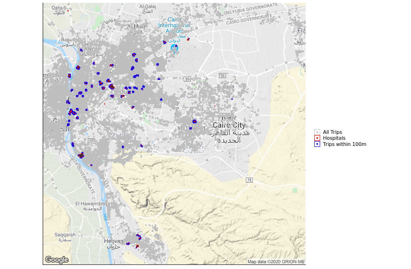
Trips to Hospitals
| Hospital 100 | Hospital 175 | Hospital 250 | |||||||
|---|---|---|---|---|---|---|---|---|---|
| (1) | (2) | (3) | (4) | (5) | (6) | (7) | (8) | (9) | |
| Overall | Female | Male | Overall | Female | Male | Overall | Female | Male | |
| Price X 75% | 11.31*** | 10.71** | 11.73*** | 21.45*** | 15.85** | 25.91*** | 28.83*** | 26.15*** | 31.13*** |
| (3.05) | (4.40) | (4.20) | (4.94) | (7.12) | (6.84) | (5.96) | (9.23) | (7.79) | |
| Price X 50% | 18.13*** | 23.67*** | 13.49*** | 32.87*** | 37.11*** | 29.35*** | 50.55*** | 52.98*** | 48.54*** |
| (3.34) | (5.00) | (4.41) | (5.07) | (7.38) | (6.89) | (6.31) | (9.05) | (8.69) | |
| Constant | 7.21*** | 6.16*** | 8.08*** | 13.62*** | 14.49*** | 12.94*** | 19.31*** | 21.40*** | 17.62*** |
| (1.50) | (1.66) | (2.35) | (2.40) | (3.99) | (2.92) | (2.74) | (4.56) | (3.35) | |
| Observations | 16452 | 7272 | 9168 | 16452 | 7272 | 9168 | 16452 | 7272 | 9168 |
Notes: The table reports the impacts of the two treatment arms on the weekly number of trips times 100 that started or finished close to a hospital taken on Uber. Columns (1), (2), & (3) report trips that are taken in a range of 100 meters from a hospital. Columns (4), (5), & (6) report trips that are taken in a range of 175 meters. Columns (7), (8), & (9) report trips that are taken in a range of 250 meters. Regressions include strata, cohort and follow-up round fixed effects as well as controls chosen using a double-post-lasso procedure. Standard errors clustered at the individual level in parentheses. Significance: *.10;**.05; ***.01.
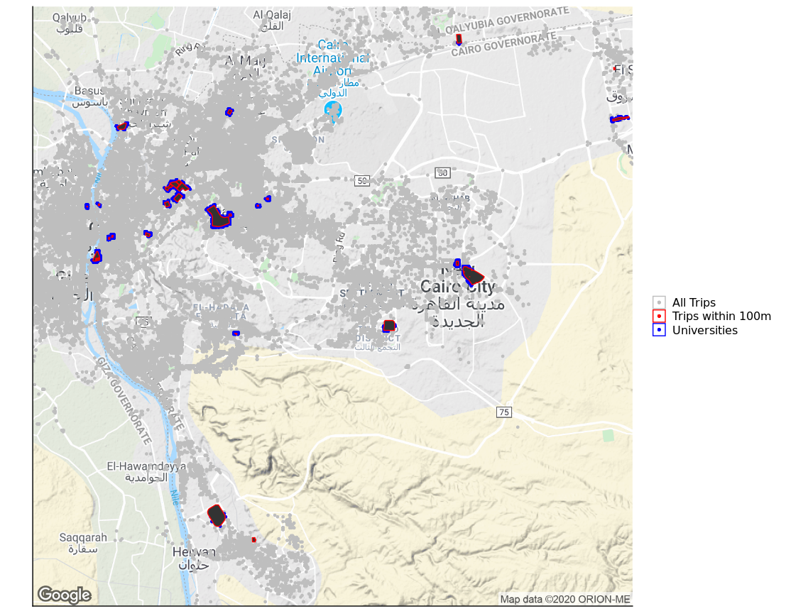
Trips to Universities
| University 100 | University 175 | University 250 | |||||||
|---|---|---|---|---|---|---|---|---|---|
| (1) | (2) | (3) | (4) | (5) | (6) | (7) | (8) | (9) | |
| Overall | Female | Male | Overall | Female | Male | Overall | Female | Male | |
| Price X 75% | 5.27** | 8.33** | 2.80* | 10.74*** | 11.90** | 9.86*** | 14.72*** | 13.88** | 15.48*** |
| (2.06) | (4.12) | (1.63) | (3.01) | (5.27) | (3.34) | (3.72) | (6.04) | (4.55) | |
| Price X 50% | 14.60*** | 21.49*** | 9.14*** | 24.25*** | 26.85*** | 22.25*** | 34.76*** | 38.97*** | 31.56*** |
| (3.22) | (6.25) | (2.91) | (4.58) | (7.03) | (5.98) | (5.53) | (8.66) | (7.12) | |
| Constant | 5.22*** | 5.59*** | 4.96*** | 7.73*** | 9.23*** | 6.54*** | 10.55*** | 12.59*** | 8.91*** |
| (0.88) | (1.33) | (1.19) | (1.18) | (2.03) | (1.42) | (1.49) | (2.45) | (1.83) | |
| Observations | 16452 | 7272 | 9168 | 16452 | 7272 | 9168 | 16452 | 7272 | 9168 |
Notes: The table reports the impacts of the two treatment arms on the weekly number of trips times 100 that started or finished close to a university taken on Uber. Columns (1), (2), & (3) report trips that are taken in a range of 100 meters from an university. Columns (4), (5), & (6) report trips that are taken in a range of 175 meters. Columns (7), (8), & (9) report trips that are taken in a range of 250 meters. Regressions include strata, cohort and follow-up round fixed effects as well as controls chosen using a double-post-lasso procedure. Standard errors clustered at the individual level in parentheses. Significance: *.10;**.05; ***.01.
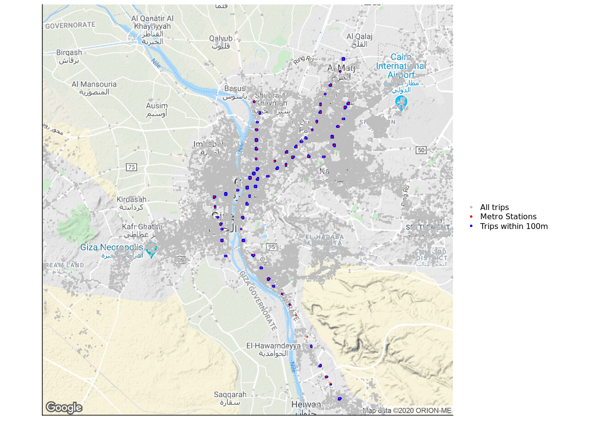
Trips to Metro Stations
| Metro 100 | Metro 175 | Metro 250 | |||||||
|---|---|---|---|---|---|---|---|---|---|
| (1) | (2) | (3) | (4) | (5) | (6) | (7) | (8) | (9) | |
| Overall | Female | Male | Overall | Female | Male | Overall | Female | Male | |
| Price X 75% | 11.17*** | 4.80*** | 16.23** | 18.19*** | 10.77*** | 24.00*** | 30.71*** | 25.27*** | 34.82*** |
| (4.03) | (1.49) | (7.15) | (4.63) | (3.01) | (7.94) | (6.27) | (6.55) | (9.94) | |
| Price X 50% | 11.86*** | 13.74*** | 10.36*** | 22.70*** | 21.68*** | 22.83*** | 37.12*** | 37.97*** | 35.73*** |
| (1.81) | (3.05) | (2.18) | (3.11) | (3.81) | (4.64) | (4.80) | (5.49) | (7.42) | |
| Constant | 4.72*** | 4.77*** | 4.69*** | 8.81*** | 8.44*** | 9.14*** | 15.73*** | 12.22*** | 18.64*** |
| (0.65) | (0.87) | (0.98) | (0.99) | (1.23) | (1.55) | (2.20) | (1.76) | (3.77) | |
| Observations | 16452 | 7272 | 9168 | 16452 | 7272 | 9168 | 16452 | 7272 | 9168 |
Notes: The table reports the impacts of the two treatment arms on the weekly number of trips times 100 that started or finished close to a metro station taken on Uber. Columns (1), (2), & (3) report trips that are taken in a range of 100 meters from a metro station. Columns (4), (5), & (6) report trips that are taken in a range of 175 meters. Columns (7), (8), & (9) report trips that are taken in a range of 250 meters. Regressions include strata, cohort and follow-up round fixed effects as well as controls chosen using a double-post-lasso procedure. Standard errors clustered at the individual level in parentheses. Significance: *.10;**.05; ***.01.
Appendix G: Salience, Treatment Length and Persistence
Salience, Length and Persistence Appendix G
It is possible that our pre-announced price reductions affected the salience of discounted Uber services, leading to increased utilization due to the attention our study brings to travel as opposed to the price effects alone. In order to better disentangle the experimental effect of the price change from the salience and length of announced discounts, we implemented two separate 1-week experiments with additional waves of participants. It is also possible that the treatment led to a sustained change in rider behavior after the price reductions were removed. We analyze that behavior further below.
Experiments on the Salience and Length of Treatment
In the first auxiliary experiment, we split the sample into 3 treatment groups (50% price reduction, 10% price reduction, control) and held all elements of the experimental protocol constant aside from the length of the intervention.[51] Participants were sent an email telling them that they were enrolled in the study, and that they would get a 1 week subsidy based on their treatment group (as opposed to the 3 months in the main experiment).
In the second auxiliary experiment, we split a different sample into 3 treatment groups (50% price reduction, 10% price reduction, control) but instead of informing the participants of their impending discount we simply applied the discount to their accounts automatically for 1 week. These individuals did not know in advance that they would have a price reduction during this time, nor did they know how long the price reduction would continue for. This experiment deviates from the main experiment in two ways: (1) in the length of the subsidy (i.e. 1 week vs 3 months) and (2) in the salience of the subsidy (pre-announced vs unannounced).
Table G.1 reports the results of these two experiments alongside estimates of effects from the first week of the main experiment. We assess the importance of salience by comparing impacts on Uber utilization for the 10% treatment group in columns 3 & 4 versus columns 5 & 6. If it were the case that prior knowledge of the discount was leading to strategic overuse of Uber during the 1 week of the discount (e.g. moving up travel they were planning to take in the future to benefit from the discount), we would expect greater increases among participants in the pre-announced experiment relative to those in the unannounced experiment. Instead, we find that the effects on weekly kilometers are nearly the same across the two experiments, while the number of trips is somewhat smaller but not statistically different in the pre-announced experiment. Even without strategic overuse, bringing attention to the subsidy could have led to additional utilization due to salience effects. We do not find any evidence to support this hypothesis.
We evaluate the effect of knowledge of the 3-month experimental treatment by comparing the impacts from the 1-week experiments to the impacts from the first week of our main experiment. The point estimate for weekly kilometers from the 50% price reduction is 0.65 in the main experiment versus 0.77 in the 1-week experiment. These estimates are statistically equivalent. Hence, it does not appear that intervention length has an important impact on the findings reported in our main experiment.
Experiments on the Length and Salience of the Price Reduction
| Long Experiment 1st Week | Preannounced Short Experiment | Unannounced Short Experiment | ||||
|---|---|---|---|---|---|---|
| (1) | (2) | (3) | (4) | (5) | (6) | |
| Weekly KM | Trips | Weekly KM | Trips | Weekly KM | Trips | |
| Price X 90% | 0.41* | 0.38 | 0.44* | 0.51 | ||
| (0.19) | (0.24) | (0.18) | (0.32) | |||
| Price X 90% * Male | -0.24 | -0.21 | -0.46 | -0.35 | ||
| (0.25) | (0.33) | (0.26) | (0.45) | |||
| Price X 75% | 0.29* | 0.86*** | ||||
| (0.17) | (0.30) | |||||
| Price X 75% * Male | 0.01 | -0.12 | ||||
| (0.24) | (0.42) | |||||
| Price X 50% | 0.65*** | 2.11*** | 0.77*** | 1.45*** | ||
| (0.17) | (0.37) | (0.19) | (0.36) | |||
| Price X 50% * Male | -0.07 | -0.80* | 0.04 | 0.79 | ||
| (0.24) | (0.47) | (0.27) | (0.56) | |||
| Observations | 1370 | 1370 | 1000 | 1000 | 1500 | 1500 |
| Control Mean (Levels) | 22.9 | 2.6 | 13.4 | 2.0 | 20.4 | 2.2 |
| Control Mean for Men | 20.9 | 2.2 | 18.7 | 2.2 | 21.4 | 2.1 |
| Panel B: Pooled Effects | ||||||
|---|---|---|---|---|---|---|
| Long Experiment 1st Week | Preannounced Short Experiment | Unannounced Short Experiment | ||||
| (1) | (2) | (3) | (4) | (5) | (6) | |
| Weekly KM | Trips | Weekly KM | Trips | Weekly KM | Trips | |
| Treatment | 1.43^{***} | 3.77^{***} | 2.76^{**} | 2.58 | 1.55^{***} | 3.72^{***} |
| (0.27) | (0.54) | (1.26) | (1.66) | (0.26) | (0.56) | |
| Observations | 1,370 | 1,370 | 1,000 | 1,000 | 1,500 | 1,500 |
| Control Mean | 21.9 | 2.4 | 16.05 | 2.1 | 20.7 | 2.1 |
Notes: Top panel reports the full set of estimates from the fully interacted model, whereas bottom panel reports pooled treatment effects to maximize statistical power (by gender and discount level as a continuous variable). Columns (1), (3), & (5) report the impacts of the two treatment arms and their interactions with a male dummy variable, on the inverse hyperbolic sine of weekly kilometers traveled on Uber during the first week of the experiment, the pre-announced experiment and the unannounced experiment respectively. Columns (2), (4), & (6) report the same but with number of trips as the outcome variable. The bottom rows report the control means in levels and split by gender. Regressions include strata, cohort and follow-up round fixed effects as well as controls chosen using a double-post-lasso procedure in columns (1) and (2). Pairwise statistical tests of coefficients in Panel B all fail to reject equality (comparing columsn 1,3,5 and 2,4,6). Standard errors clustered at the individual level in parentheses. Significance: *.10; **.05; ***.01.
Longer Term Impacts on Uber Utilization
While the subsidies provided to the participants in our study changed their Uber usage during the 12 weeks of the intervention, it is unclear how their usage would change after discontinuing the subsidies. It is possible that individuals go back to their pre-treatment utilization levels, but it also possible that individuals have learned how to better optimize their mobility choices now that they have additional experience with Uber and decide to use it more than they did before. On the other hand, they may have become used to having access to Uber at a lower price, changing their reference points for acceptable costs, and decrease their Uber usage after the end of the intervention due to the relative increase in price.
Using Uber administrative data, we can estimate the impact of the treatments on rider behavior after the subsidies are removed. Table G.2 reports the impacts on total weekly kilometers traveled on Uber and the number of weekly trips taken during the 12 weeks after the end of the intervention (weeks 13-24 after randomization). We find that those in treatment use Uber much more than those in control, an increase of 0.55 IHS-points for the 25% treatment group (a 73% increase), and an increase of 0.60 IHS-points for those in the 50% group (an 82% increase). While this is much smaller than the impact from the actual price reductions, these estimates are both statistically and economically significant. Point estimates suggest that the persistence of effects for participants in the 50% group is lower than for those in the 25% group. One possible explanation is that participants anchored their reference point at the 50% price level, making the price increase after the end of the intervention larger compared to those in the 25% group. However, we note that treatment effects are less precisely estimated than effects during the treatment period and that differences between groups are not statistically significant.
Persistence of Uber Utilization After Study
| Weekly KM on Uber (IHS) | Weekly Trips on Uber | |||
|---|---|---|---|---|
| (1) | (2) | (3) | (4) | |
| Price X 75% | 0.55*** | 0.92*** | 0.77*** | 1.18*** |
| (0.13) | (0.24) | (0.23) | (0.40) | |
| Price X 75% * Male | -0.50* | -0.50 | ||
| (0.28) | (0.47) | |||
| Price X 50% | 0.60*** | 0.75*** | 0.80*** | 0.68 |
| (0.13) | (0.25) | (0.20) | (0.43) | |
| Price X 50% * Male | -0.19 | 0.04 | ||
| (0.29) | (0.48) | |||
| Observations | 4251 | 4251 | 4251 | 4251 |
| Control Group Mean Levels | 12.1 | 13.9 | 1.3 | 1.6 |
| Control Group Mean Levels (Male) | 11.4 | 1.3 |
Notes: Column (1) reports the impacts of the two treatment arms on the inverse hyperbolic sine of weekly kilometers traveled on Uber after the experiment is finished. Column (2) reports the results from a specification that interacts a dummy variable for men, showcasing the differential impact the treatments have for that subgroup. Columns (3) & (4) report the estimates from a regression on the weekly number of trips taken on Uber (in levels). The bottom rows report the control means in both IHS and levels for each group in Columns (1) & (3), and split the means by the interacted and non-interacted groups in columns (2) & (4). Regressions include controls chosen using a double-post-lasso procedure. Regressions include strata, cohort and follow-up round fixed effects as well as controls chosen using a double-post-lasso procedure. Standard errors clustered at the individual level in parentheses. Significance: *.10; **.05; ***.01.
Appendix H: Estimates of Treatment Effects Omitting Lasso-Based Controls
Controlling for Baseline Value Appendix H
In this section, we report estimates for all main tables using regressions that control for the baseline value of the outcome variable instead of the set of controls selected when using the double post-lasso procedure developed by Belloni et al. (2014). We use this procedure in the main paper because it can help improve power by optimally selecting the baseline controls that minimize residual variance of the outcome variable. We find no evidence of sensitivity to the inclusion of these controls, although the precision of estimates often increases when we utilize the double post-lasso procedure, in line with their theoretical purpose.
We included 34 variables for the lasso to utilize: Gender, total travel, travel on Uber, marital status, work status, car ownership, motorcycle ownership, aspects of their longest trip in the day before the survey (safety, time, cost), feelings of safety on 6 different transport modes, education, and an interaction of all of these variables with a dummy variable for male.
The procedure selects controls for each regression separately, and so listing out the chosen controls for each table would be messy. We find that the most common variables that are chosen are total distance traveled, distance traveled on Uber, education, income and safety perceptions.
Impacts of Uber Subsidies on Uber Utilization
| Weekly KM on Uber (IHS) | Weekly Trips on Uber | |||
|---|---|---|---|---|
| (1) | (2) | (3) | (4) | |
| Price X 75% | 1.00*** | 1.08*** | 1.73*** | 1.98*** |
| (0.08) | (0.12) | (0.15) | (0.21) | |
| Price X 75% * Male | -0.15 | -0.44 | ||
| (0.16) | (0.30) | |||
| Price X 50% | 1.69*** | 1.84*** | 3.68*** | 4.20*** |
| (0.08) | (0.12) | (0.20) | (0.31) | |
| Price X 50% * Male | -0.27 | -0.92** | ||
| (0.16) | (0.41) | |||
| Observations | 16440 | 16440 | 16440 | 16440 |
| Control Group Mean Levels | 13.6 | 14.1 | 1.5 | 1.6 |
| Control Group Mean Levels (Male) | 13.2 | 1.5 |
Notes: Column (1) reports the impacts of the two treatment arms on the inverse hyperbolic sine of weekly kilometers traveled on Uber. Column (2) reports the results from a specification that interacts a dummy variable for men, showcasing the differential impact the treatments have for that subgroup. Columns (3) & (4) report the estimates from a regression on the weekly number of trips taken on Uber (in levels). The bottom rows of Panel A report the control means in levels for each group in Columns (1) & (3), and split the means by gender in columns (2) & (4). Regressions include strata, cohort and follow-up round fixed effects as well as baseline value of the outcome variable as control. Standard errors clustered at the individual level in parentheses. Significance: *.10; **.05; ***.01.
Experiments on the Length and Salience of the Price Treatment
| Unannounced Short Experiment | Preannounced Short Experiment | Long Experiment 1st Week | ||||
|---|---|---|---|---|---|---|
| (1) | (2) | (3) | (4) | (5) | (6) | |
| Weekly KM | Trips | Weekly KM | Trips | Weekly KM | Trips | |
| Price X 90% | 0.42** | 0.49 | 0.42** | 0.38 | ||
| (0.18) | (0.32) | (0.19) | (0.24) | |||
| Price X 90% * Male | -0.44* | -0.32 | -0.25 | -0.22 | ||
| (0.26) | (0.45) | (0.25) | (0.33) | |||
| Price X 75% | 0.32* | 0.88** | ||||
| (0.20) | (0.34) | |||||
| Price X 75% * Male | 0.19 | 0.24 | ||||
| (0.27) | (0.49) | |||||
| Price X 50% | 0.77*** | 1.44*** | 0.84*** | 2.49*** | ||
| (0.19) | (0.36) | (0.20) | (0.43) | |||
| Price X 50% * Male | 0.04 | 0.80 | -0.23 | -1.08** | ||
| (0.27) | (0.56) | (0.27) | (0.55) | |||
| Observations | 1500 | 1500 | 1000 | 1000 | 1370 | 1370 |
| Control Mean | 20.4 | 2.2 | 13.4 | 2.0 | 22.9 | 2.6 |
| Control Mean (Male) | 21.4 | 2.1 | 18.7 | 2.2 | 20.9 | 2.2 |
Notes: Columns (1), (3), & (5) report the impacts of the two treatment arms and their interactions with a male dummy variable, on the inverse hyperbolic sine of weekly kilometers traveled on Uber during the unannounced experiment respectively , the pre-announced experiment and the first week of the experiment. Columns (2), (4), & (6) report the same but with number of trips as the outcome variable. The bottom rows report the control means in levels and split by gender. Regressions include strata, cohort and follow-up round fixed effects as well as baseline value of the outcome variable as control. Standard errors clustered at the individual level in parentheses. Significance: *.10; **.05; ***.01.
Impacts in Total Mobility
| Total KM Past 3 Days (IHS) | ||
|---|---|---|
| (1) | (2) | |
| Price X 75% | 0.10 | 0.17 |
| (0.09) | (0.14) | |
| Price X 75% * Male | -0.12 | |
| (0.19) | ||
| Price X 50% | 0.36*** | 0.49*** |
| (0.08) | (0.12) | |
| Price X 50% * Male | -0.26 | |
| (0.17) | ||
| Observations | 3476 | 3476 |
| Control Group Mean Levels | 88.0 | 62.0 |
| Control Group Mean Levels (Male) | 111.9 |
Notes: Column (1) reports the impacts of the two treatment arms on the inverse hyperbolic sine of total kilometers traveled in the three days prior to our follow-up survey as reported by Google Maps’ “Timeline" feature. Column (2) reports the results from a specification that interacts a dummy variable for men, showcasing the differential impact the treatments have for that subgroup. The bottom rows report the control means in levels and split the means by the interacted group, and non-interacted groups in Columns (2).Regressions include strata, cohort and follow-up round fixed effects as well as baseline value of the outcome variable as control. Standard errors clustered at the individual level in parentheses. Significance: *.10; **.05; ***.01.
Impacts on Mode Used for Longest Trip
| Metro | Bus | Taxi | Uber | Car | ||||||
|---|---|---|---|---|---|---|---|---|---|---|
| (1) | (2) | (3) | (4) | (5) | (6) | (7) | (8) | (9) | (10) | |
| Price X 75% | -0.01 | -0.02 | -0.06** | -0.04 | -0.02** | -0.03** | 0.10*** | 0.10*** | -0.01 | -0.01 |
| (0.01) | (0.02) | (0.03) | (0.04) | (0.01) | (0.01) | (0.02) | (0.04) | (0.03) | (0.04) | |
| Price X 75% * Male | 0.03 | -0.03 | 0.02 | 0.00 | -0.01 | |||||
| (0.03) | (0.05) | (0.01) | (0.05) | (0.05) | ||||||
| Price X 50% | 0.00 | -0.01 | -0.1*** | -0.1*** | -0.02** | -0.03** | 0.13*** | 0.15*** | -0.02 | 0.00 |
| (0.01) | (0.02) | (0.03) | (0.04) | (0.01) | (0.01) | (0.02) | (0.04) | (0.03) | (0.04) | |
| Price X 50% * Male | 0.02 | 0.02 | 0.02 | -0.03 | -0.03 | |||||
| (0.03) | (0.05) | (0.01) | (0.05) | (0.05) | ||||||
| Observations | 3186 | 3186 | 3186 | 3186 | 3186 | 3186 | 3186 | 3186 | 3186 | 3186 |
| Control Group Mean Levels | 0.1 | 0.1 | 0.3 | 0.3 | 0.0 | 0.0 | 0.2 | 0.3 | 0.3 | 0.3 |
| Control Group Mean Levels (Male) | 0.1 | 0.4 | 0.0 | 0.2 | 0.3 |
Notes: This table reports the coefficients from a regression on a binary outcome that takes the value 1 if the individual reported taking that mode of transportation for their longest trip the day our follow-up survey. Even numbered columns report the results from a specification that interacts treatment with a dummy variable for men. The bottom rows report the control means in levels, split by gender in even numbered columns. Regressions include strata, cohort and follow-up round fixed effects as well as baseline value of the outcome variable as control. Standard errors clustered at the individual level in parentheses. Significance: *.10; **.05; ***.01.
Impacts on Reported Safety on Recent Trips
| Feeling on Longest Trip Yesterday | ||
|---|---|---|
| 5=Very Safe, 1=Very Unsafe | ||
| (1) | (2) | |
| Price X 75% | 0.07 | 0.16* |
| (0.06) | (0.09) | |
| Price X 75% * Male | -0.16 | |
| (0.12) | ||
| Price X 50% | 0.11* | 0.20** |
| (0.06) | (0.09) | |
| Price X 50% * Male | -0.18 | |
| (0.11) | ||
| Observations | 3101 | 3101 |
| Control Group Mean Levels | 4.0 | 3.9 |
| Control Group Mean Levels (Male) | 4.1 |
Notes:Column (1) reports the impacts of the two treatment arms on the reported level of safety felt during the longest trip taken by the individual during the day prior to the follow-up survey. Column (2) reports the results from a specification that interacts treatment with a dummy variable for men. The bottom rows report the control means in levels, split by gender in Column (2). The bottom rows report the control means in levels, split by gender in even numbered columns. Regressions include strata, cohort and follow-up round fixed effects as well as baseline value of the outcome variable as control. Standard errors clustered at the individual level in parentheses. Significance: *.10; **.05; ***.01.
Effect on Baseline Bus Riders
| Panel A:Weekly Uber Usage (KM) | Weekly KM on Uber(IHS) | Weekly KM on Uber(IHS) | ||||
|---|---|---|---|---|---|---|
| Perceive Bus as Unsafe | ||||||
| (1) | (2) | (3) | (4) | (5) | (6) | |
| Overall | Female | Male | Overall | Female | Male | |
| Price X 75% | 1.08*** | 1.11*** | 1.06*** | 1.07*** | 1.24*** | 0.90*** |
| (0.09) | (0.14) | (0.12) | (0.15) | (0.21) | (0.22) | |
| Price X 75% * Bus User | -0.29* | -0.06 | -0.43* | -0.36 | -0.34 | -0.17 |
| (0.16) | (0.24) | (0.22) | (0.33) | (0.43) | (0.48) | |
| Price X 50% | 1.69*** | 1.70*** | 1.69*** | 1.59*** | 1.77*** | 1.44*** |
| (0.10) | (0.14) | (0.13) | (0.15) | (0.19) | (0.22) | |
| Price X 50% * Bus User | -0.02 | 0.57** | -0.38 | -0.03 | 1.10** | -0.56 |
| (0.17) | (0.24) | (0.23) | (0.33) | (0.46) | (0.42) | |
| Observations | 16440 | 7272 | 9168 | 6012 | 3336 | 2676 |
| Control Group Mean Levels | 25.5 | 25.7 | 25.4 | 25.9 | 27.5 | 23.5 |
| Control Group Mean Levels (Bus User) | 13.4 | 14.0 | 13.1 | 12.6 | 6.2 | 15.6 |
| Panel B:Total Mobility (KM) | ||||||
| Total Mobility (KM) in past 3 days(IHS) | Total Mobility (KM) in past 3 days(IHS) | |||||
| Perceive Bus as Unsafe | ||||||
| (1) | (2) | (3) | (4) | (5) | (6) | |
| Overall | Female | Male | Overall | Female | Male | |
| Price X 75% | 0.10 | 0.18 | -0.04 | 0.03 | 0.02 | 0.03 |
| (0.12) | (0.17) | (0.15) | (0.17) | (0.23) | (0.24) | |
| Price X 75% * Bus User | 0.02 | 0.04 | 0.15 | 0.64 | 0.91 | 0.72 |
| (0.21) | (0.32) | (0.26) | (0.35) | (0.60) | (0.41) | |
| Price X 50% | 0.37*** | 0.52*** | 0.21 | 0.23 | 0.43* | -0.12 |
| (0.11) | (0.15) | (0.14) | (0.15) | (0.18) | (0.25) | |
| Price X 50% * Bus User | -0.04 | -0.12 | 0.12 | 0.50 | 0.79 | 0.62 |
| (0.18) | (0.29) | (0.22) | (0.31) | (0.57) | (0.36) | |
| Observations | 3476 | 1666 | 1810 | 1313 | 780 | 533 |
| Control Group Mean Levels | 93.8 | 61.0 | 130.2 | 95.7 | 67.8 | 142.9 |
| Control Group Mean Levels (Bus User) | 75.6 | 64.8 | 82.1 | 63.1 | 52.6 | 68.6 |
Notes: Panel A: Columns (1), (2), & (3) report impacts on the inverse hyperbolic sine of weekly kilometers traveled on Uber in a specification that interacts the treatment with a dummy variable that takes the value of 1 if the individual reports at baseline that the longest trip took in the previous day was using a bus and 0 otherwise. Columns (4), (5), & (6) in panel A report the result for a specification that includes only people who perceived the bus as unsafe in the baseline survey. Panel B reproduces the same regressions but with total kilometers traveled as the outcome variable. The bottom rows in each panel report the control means in levels, split by if they were bus users at baseline. Regressions include strata, cohort and follow-up round fixed effects as well as baseline value of the outcome variable as control. Standard errors clustered at the individual level in parentheses. Significance: *.10; **.05; ***.01.
Labor Market Outcomes Appendix I
Appendix I: Effects on Short-Term Labor Market Outcomes
This section reports on the impacts of reductions in the cost of ride-hailing services on labor market impacts. A price decrease could improve the ability of job seekers to better match with existing vacancies. Previous studies, such as Abebe et al. (2021); Franklin (2018); Abebe et al. (2021); Bryan et al. (2014) and Phillips (2014), provide evidence that travel subsidies can improve employment outcomes. Other work has shown the importance of safety on female education and labor market choices in developing country cities (Kondylis et al. (2020); Borker (2018); Jayachandran (2019)).
Table H.7 reports impacts on job search and work status. We stratified our sample by job search status and interact search status with treatment in this table. The main effects are reported for individuals who were searching for a job at baseline. Overall, we find little evidence that these subsidies had substantial effects on search behavior or employment for either gender across the 3-month study period. We find that among individuals who were searching for a job at baseline, there is a one percentage point decrease in whether those in the 25% treatment group are currently working relative to control, and a three percentage point decrease in the 50% subsidy group. These null effects are precisely estimated, with standard errors of 3 percentage points.
These results contribute to a growing literature on the labor market impacts of transport subsidies, much of which has found that transport frictions are an important part of the reason why job seekers are not matching with employers. The present study provides larger subsidies, over a longer period, and delivers transport services using a highly flexible ride-hailing platform. The intervention generates large effects on mobility yet we can rule out large labor market effects (in the short-run). Our findings reflect effects on a higher income sample than the earlier studies, implying that transport frictions in the job search phase may interact in important ways with capital constraints in low income countries.
Labor Market Impacts
| Searching | Apply | Currently Working | |||||||
|---|---|---|---|---|---|---|---|---|---|
| (1) | (2) | (3) | (4) | (5) | (6) | (7) | (8) | (9) | |
| Overall | Female | Male | Overall | Female | Male | Overall | Female | Male | |
| Price X 75% | -0.03 | 0.02 | -0.04 | -0.47** | -0.32 | -0.50* | -0.01 | 0.02 | -0.01 |
| (0.04) | (0.08) | (0.05) | (0.23) | (0.34) | (0.30) | (0.03) | (0.07) | (0.04) | |
| Price X 75% * Not Searching | 0.08 | 0.02 | 0.10 | 0.60** | 0.39 | 0.67** | -0.06 | -0.09 | |
| (0.05) | (0.08) | (0.06) | (0.25) | (0.36) | (0.32) | (0.06) | (0.08) | ||
| Price X 50% | 0.02 | -0.04 | 0.05 | -0.01 | 0.60 | -0.20 | -0.03 | -0.01 | -0.01 |
| (0.04) | (0.07) | (0.05) | (0.30) | (0.68) | (0.32) | (0.03) | (0.08) | (0.03) | |
| Price X 50% * Not Searching | -0.01 | 0.02 | -0.01 | 0.07 | -0.63 | 0.34 | 0.03 | 0.01 | |
| (0.04) | (0.08) | (0.06) | (0.30) | (0.70) | (0.33) | (0.05) | (0.09) | ||
| Observations | 3195 | 1501 | 1692 | 3193 | 1500 | 1691 | 1643 | 959 | 684 |
| Control Group Mean Levels | 0.50 | 0.43 | 0.52 | 1.28 | 0.94 | 1.43 | 0.80 | 0.69 | 0.85 |
| Control Group Mean Levels (N.S.) | 0.07 | 0.08 | 0.07 | 0.08 | 0.09 | 0.05 | 0.66 | 0.66 | 1.00 |
Notes: Columns (1), (2), & (3) report the impact of treatments on a binary variable that is equal to 1 if the individual reports that they are searching for work during the follow-up survey. The regression specification includes treatment interacted with a dummy equal to 1 if the individual was not searching for work at baseline. Columns (4), (5), & (6) estimate the impacts on the number of jobs applied to, while columns (7), (8), & (9) estimate the impacts on if the individuals are currently working at the time of the follow-up survey. The bottom rows report the control means in levels, split by if they were searching for a job at baseline (N.S. = “Not Searching”). There is no variation in responses for men who were not searching for a job at baseline in column 9 and so those interaction cells are intentionally left empty (they are all currently working). Regressions include strata, cohort and follow-up round fixed effects as well as controls chosen using a double-post-lasso procedure.
Standard errors clustered at the individual level in parentheses. Significance: *.10; **.05; ***.01.
Appendix J: Adjustments for COVID-19
COVID-19 Appendix J
Our budget allowed us to enroll 1,500 participants, but our last cohort was impacted by the lock-down associated with COVID-19. Since mobility behavior was greatly affected by this unusual worldwide event, we drop this cohort from our main analysis. The sample used in our main analysis consists of 1,373 participants, though we do have administrative data and some follow-up data on the final cohort. Including the final cohort in our analysis does not substantially affect our results, though estimates are slightly attenuated as a result of reductions in mobility levels for all participants in that cohort. COVID-19 also negatively impacted our intended 6-month follow-up survey, which was designed to collect additional data on overall mobility and labor market outcomes three months after the completion of the experiment. We had collected those data for one third of the sample by the time the lock-down began. Given selection and attrition concerns, we do not report these longer-term results.
Main Results including Cohort Affected by COVID-19
| Weekly KM on Uber (IHS) | Weekly Trips on Uber | Total KM Past 3 Days | ||||
|---|---|---|---|---|---|---|
| (1) | (2) | (3) | (4) | (5) | (6) | |
| Price X 75% | 0.94*** | 1.03*** | 1.65*** | 1.79*** | 0.14 | 0.19 |
| (0.07) | (0.11) | (0.14) | (0.20) | (0.09) | (0.13) | |
| Price X 75% * Male | -0.17 | -0.25 | -0.15 | |||
| (0.14) | (0.29) | (0.17) | ||||
| Price X 50% | 1.60*** | 1.68*** | 3.44*** | 3.73*** | 0.39*** | 0.50*** |
| (0.08) | (0.11) | (0.19) | (0.28) | (0.08) | (0.11) | |
| Price X 50% * Male | -0.15 | -0.55 | -0.25 | |||
| (0.15) | (0.37) | (0.15) | ||||
| Observations | 17964 | 17964 | 17964 | 17964 | 3670 | 3670 |
| Control Group Mean Levels | 12.1 | 13.9 | 1.3 | 1.6 | 55.8 | 34.8 |
| Control Group Mean Levels (Male) | 11.4 | 1.3 | 75.1 |
Notes: Column (1) reports the impacts of the two treatment arms on the inverse hyperbolic sine of weekly kilometers traveled on Uber. Column (2) reports the results from a specification that interacts a dummy variable for men, showcasing the differential impact the treatments have for that subgroup. Columns (3) & (4) report the estimates from a regression on the weekly number of trips taken on Uber (in levels). Columns (5) & (6) report the impacts on the inverse hyperbolic sine of total kilometers traveled in the three days prior to our follow-up survey as reported by Google Maps’ “Timeline” feature. The bottom rows report the control means in levels and split by gender in Columns (2), (4), & (6). Regressions include strata, cohort and follow-up round fixed effects as well as controls chosen using a double-post-lasso procedure. Standard errors clustered at the individual level in parentheses. Significance: *.10; **.05; ***.01.
Appendix K: Model Derivations & Sample Moments
Derivations & Moments Appendix K
This section outlines how we use our model to estimate welfare. In the first part we show how we derive an expression for the change in $V(p)$, the value of utility at price “p”. In the second part we outline the different moments we use from our experiment and the academic literature to estimate our model. \\
From equation 2 in section 5, we recall the utility maximization problem as:
We re-write the problem as:
The first order conditions of this maximization problem are:
We then apply the envelope theorem to find $\frac{\partial V}{\partial c(P,1)}$. Starting from the budget constraint, we have:
Taking the total differential:
The total differential of utility at the optimum is:
Since $U_{Q_M}(Q_M,Y) = \lambda c(P,1)$ and $U_Y(Q,Y) = \lambda$, we substitute these into the expression:
Next, substituting $\partial Y = -Q_M.\partial c(P,1) - c(P,1) . \partial Q_M$:
Distributing $\lambda$:
Note that $\lambda . c(P,1) . \partial Q_M$ and $-\lambda c(P,1) \partial Q_M$ cancel out, leaving:
Hence the solution is:
Taking the second derivative, we get:
We can express the change in welfare as a change in the price of each good in the following way[52]:
We can then approximate the solution to second order in terms of percentage changes:
From the F.O.C in the maximization problem, we know that:
In our setup, the utility function assumes CES with a congestion (i.e. time) penalty :
and so $\lambda(p)$ is equal to:
The change of $\lambda^*(p)$ with respect to price is:
Substituting the derivatives with respect to price with their corresponding elasticities provides:
Then, substituting the term from equation (4) into equation (1) provides the expression for the change in utility ($\Delta V$) to second order. We divide this value by $\lambda(p)$ to get an estimate of compensating variation. We use our experimentally identified parameters and the derived expressions to produce the values reported in Tables 6 & 7.
Sample Moments used in the Model
Here we define the moments taken from our experiment/sample for the model:
- $\epsilon_{Lcc}$ -- the experimentally identified elasticity of demand for low-occupancy travel (i.e. Car, Uber, Careem, Taxi, Toktok) with respect to the price of low-occupancy travel: -1.4.[53]
- $\epsilon_{Q_M}$ -- the experimentally identified elasticity of demand for total kilometers traveled with respect to the price of low-occupancy travel: -1.2.[54]
- $W$ -- the average income reported in our sample: 5,468EGP\slash month. We also estimate a wage of 34.2 EGP\slash hour using this and the assumption that survey respondents work 160 hours a month.
- $\frac{Q_M\cdot c(P,1)}{W}$ -- the baseline share of the budget that individuals spend on travel: 0.07.
- $Q_M$ -- the baseline quantity of total travel: 205km.
- $T$ -- the average time it takes for individuals to travel one kilometer in our sample: 3.06 minutes (0.051 hours).
- $C$ -- the average cost per kilometer across the different modes of transportation in our sample: 6.19EGP \slash KM.
Here we define the moments taken from the literature for the model:
- $VOT$ -- We initially include VOT as a parameter that is estimated by the model. We then calculate the model-implied VOT as $(dQ/dT) / (dQ/dP)$ which can be expressed as $(\frac{\varepsilon_{Q,T}}{\varepsilon_{Q,P}})*(\frac{P}{T_0})$. Based on our estimates, the model-implied VOT is 95% of hourly wage. We then calibrate the model using two distinct estimates of VOT from the literature -- 75% of the hourly wage from (Goldszmidt et al. (2020)) & 150% of the hourly wage from (Parry and Timilsina (2015)).
- Hence $VOT=75%\cdot wage \cdot T \cdot C$ or $150%\cdot wage \cdot T \cdot C$
The figure below illustrates how our estimates for private benefits change across a range of $VoT$ estimates, including 100% and 125% of the hourly wage.
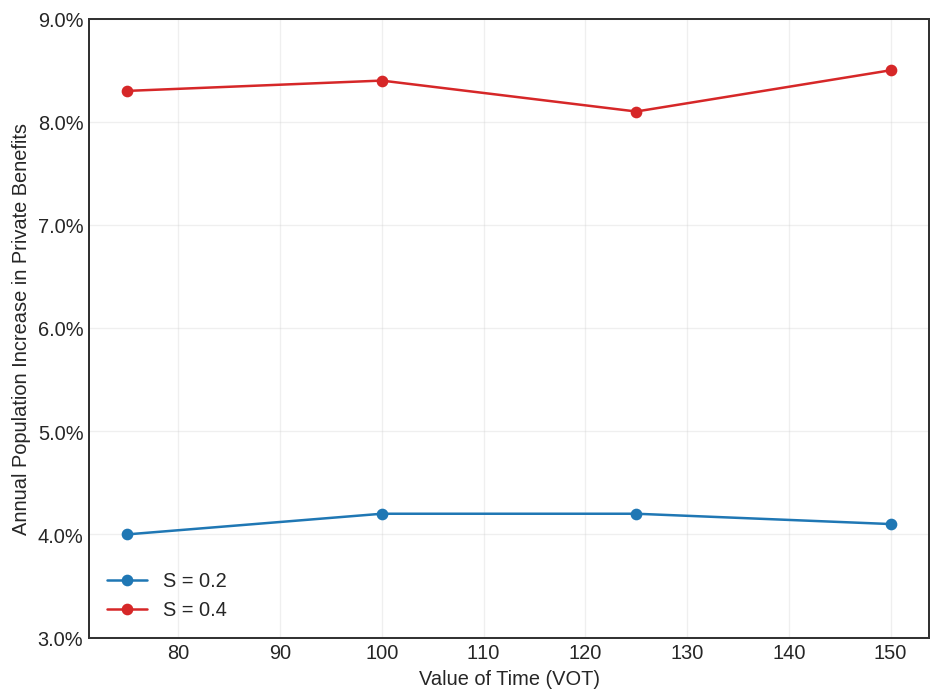
- $S$ -- the share of the population that uses ride-hailing.
- The relative contribution to congestion from 1km traveled in a high-occupancy vehicle vs. in a low-occupancy vehicle. Estimates from Authority (2017) indicate that high-occupancy vehicles contribute 0.2 as much as low-occupancy vehicles.
We consider three values: 0.2, 0.3 & 0.4. Our baseline estimate of $S=0.2$ comes from Reuters (2018), who report that 20% of the current population uses ridehailing. We consider 50% and 100% increases in that baseline share.
Appendix L: Ethics of RCT and Uber Collaboration
Ethics Appendix L
We have developed this appendix in an effort to describe the ethical considerations of this experiment, and clarify the nature of the collaboration between the researchers and Uber. We follow the framework put forth in Asiedu et al. (2021), for the sake of comparability within economics. When relevant, we quote from the main text or directly from our IRB documentation, which we did not deviate from.
- {\bf Equipoise}
- {\bf Role of Researchers with Respect to Implementation:}
- {\bf Potential Harms to Research Participants from the Interventions:}
- {\bf Potential Harms to Research Participants from Data Collection or Research Protocols}
- {\bf Potential Harms to Non-Participants:} Non-participants did not receive incentives, but were not subject to any known risk due to non-participation.
- {\bf Potential Harms to Research Staff:} Research staff running phone surveys, analyzing data, and implementing price changes on the Uber platform are not subject to any known risk.
- {\bf Scarcity:} The price treatments in this study reduced the price of Uber services for individuals assigned to treatment groups and did not negatively affect the aggregate value programs/services currently offered by Uber.
- {\bf Counterfactual Policy:} All participants in the study received incentives for participation in surveys, directly from price reductions, or both. No participants were adversely affected relative to counterfactual conditions had they opted out of the study.
- {\bf Researcher Independence:} This study was conducted through a collaboration between PIs Christensen and Osman and Uber Research. The study was conceived and designed by Christensen and Osman, who maintained full intellectual freedom throughout all stages of the project through the following:
- All experimental protocols were defined and agreed upon prior to initiating the partnership. Access to Uber administrative data and protocols for maintaining the privacy of participants were established in a legal agreement between the University of Illinois and Uber Technologies, which was executed on 10/15/2018. Uber staff never had access to any data collected outside their platform, including the data collected via participant surveys or Google Timeline.
- Research was conducted with the understanding that research design, empirical tests, and interpretation of results would be based on established methods/practices/literature in economics, irrespective of any other considerations.
- Research results were reported to Uber after the completion of analysis and shared outside the research team after completion of the working paper. Uber reserved the right to review the contents of the working paper before public release to ensure that no confidential information was shared, but did not shape or in any way influence the analysis or interpretation of results.
- {\bf Financial Conflicts of Interest:} Christensen and Osman did not receive any form of financial compensation from Uber as part of this study (nor did any assistants or staff associated with the UIUC research team). No Uber employee was named as a PI or participant in any research grant that provided funding for this project.
- {\bf Reputational Conflicts of Interest:} The research questions pursued in this study and the results described in this study are novel and different form of prior work conducted by the authors. We perceive no reputational conflicts of interest.
- {\bf Feedback to Participants or Communities:}
- {\bf Foreseeable Misuse of Research Results:}
Excerpt from Introduction: {\it Attempts to study the demand for mobility have been limited not only by the complexity of transportation markets, but also by endogeneity concerns and a lack of available micro-data on transportation behavior.
...This paper contributes to a growing empirical literature on the impact of transportation services on commuting patterns and economic activity in cities (Campante and Yanagizawa-Drott (2017); Asher and Novosad (2018); Hanna et al. (2017)). A primary challenge in this literature is that the provision and prices of transportation services are (almost) never randomly assigned. As a result, empirical efforts have focused on settings characterized by exogenous shocks in service provision (Gupta et al. (2020); Gorback (2020); Tsivanidis (2018); Gonzalez-Navarro and Turner (2018); Ahlfeldt et al. (2015); Anderson (2014)), available instruments (Severen (2018); Baum-Snow et al. (2017); Duranton and Turner (2011); Baum-Snow (2007)), and structural approaches (Heblich et al. (2020); Allen and Arkolakis (2020); Redding and Rossi-Hansberg (2017)). }
Christensen and Osman are active researchers in the project. They designed the treatment arms and managed the data collection activities and all of the data analysis.
Excerpt From IRB #19102: {\it There are no known risks other than the normal privacy risks from participation in any research study. All participants will provide consent. Initial consent will be obtained through an online form. We will send an email to individuals in the follow-up experiments to give them the opportunity to opt-out of the follow up experiment.}
Excerpt From IRB #19102: {\it Individuals will enroll in the study by providing the researchers their identifying information, including the email address that is associated with their Uber account. We will generate two unique IDs for each of these email addresses, and we will provide one of the ID/email address combinations to Uber. Uber will send us back rider data using the unique ID. Uber staff will not have access to any additional information about the participants in our study or obtain any new information at all about sample participants.}
{\it Individuals will be given unique IDs. Personal identifying information will be kept separate. Only de-identified data will ever be shared. The identity key will be kept separate from participant data, maintained in an encrypted folder on PI hard-drives, on a password protected computer.}
We intend to share our results with participants via email after our work is subject to peer-review.
The authors recognize that the results described in this paper involve research questions that are relevant for public policy and regulatory activities in ride-hailing markets. Any misinterpretation or deliberate mis-characterization of the results of this study could have implications for individuals, communities and firms affected by these markets. We dedicate Section 6 to a discussion of the limitations of the study and method and will provide de-identified data for full transparency/replicability.
Notes
Individuals volunteered to join the research program, as outlined in section 1.1 below. ↩
Google Maps’ Timeline feature is part of the Google Maps app and when activated tracks an individual’s movement throughout the day. This allows us to get high quality data on the total amount of kilometers traveled by each participant during the study period. ↩
We focus on kilometers traveled as opposed to the number of trips taken because that is the relevant metric for assessing congestion and emission externalities. We also report impacts on trips, which are similar. ↩
Relatedly, Alvarez and Argente (2020) use experiments to estimate how demand for Uber changes based on riders’ payment method, cash or credit. ↩
If surge pricing is commonly engaged during very busy periods with increased congestion, then the elasticity estimates used to compute CS may differ from the elasticities from non-surge trips. Shen (2023) suggests that ridehailing elasticities are higher in the face of congestion, which would imply that Cohen et al. (2016) estimates are upper bounds. Elasticities from surge pricing also differ from the variation we would observe from a market-wide experiment, where a change in price could affect road congestion and the effective prices of travel on outside modes (which we discuss in Section 6.2). ↩
Uber acquired Careem in 2019, but regulators approved the purchase conditional on Careem continuing to operate as an independent brand with independent management (Saba (2019)). ↩
This is somewhat lower than the share of income spent on transport in Latin American cities, where households spend between 12-15% of income on transport (Gandelman et al. (2019)). ↩
In this paper, “price reduction” refers to experimental changes to the price faced by the consumer vs. changes in the market price of Uber services. ↩
Participants were informed that price reductions would not apply to rides on Uber Select, which is a service that provides on-demand rides in luxury cars and is Uber’s most expensive option. This restriction was implemented to safeguard against the potential depletion of funds on services that were not commonly used and less relevant for the study. ↩
The response rate to the text message was about 2%, which is typical of these types of solicitations (Allcott et al. (2020); Allcott et al. (2021)). ↩
We do not observe whether the participants had read the enrollment email. The results below indicate that individuals respond to the subsidies within the first week (see Figure 1), providing evidence that the emails were seen in a timely fashion. Individuals were also cross-randomized into an information treatment. The entirety of treatment was two additional sentences in the enrollment email. One group was informed about a popular online job board that includes thousands of vacancies, and another was informed about a website that provided data on harassment risk around the city. We control for these additional treatments in our regressions, but their impacts are outside the scope of this paper. ↩
As discussed in Appendix I, we exclude the final cohort which was affected by COVID-19. Including them in our estimates does not qualitatively change the reported results. ↩
Uber engineers can identify whether people were utilizing their account to provide discounted rides for other people and reported a negligible number of rides that fit that criteria in our sample. ↩
The ‘discount display’ (strike-through) was a requirement of the Uber engineering team. While not prominent on the screen, it could possibly affect the behavior of participants. ↩
We ask about ride-hailing as a whole to capture the overall effects on ride-hailing services, which include substitution from Careem to Uber. A few companies in Cairo (such as Swvl) now provide private bus services that people reserve in advance. Mini-buses in Cairo are vehicles that are about the size of a large van and can hold about a dozen passengers. They are usually the cheapest form of transit and follow varied routes usually starting and ending at known landmarks. ↩
It is possible that part of the treatment effect is coming from making participants more cognizant of their Google Maps app and timeline and that this leads to a differential impact by treatment. But since the app is pre-installed on all Android phones and is one of the most downloaded apps on iPhone, we think any impact would be small relative to the direct treatment effect. ↩
These one-time credits have the potential to have differential impacts due to their interaction with reduced prices. On average, 1 km of travel on Uber costs approximately 6 EGP, so those in the 50% treatment could travel an additional 4 km on each credit relative to control. A conservative upper bound estimate of this impact would be 20 km over the study period. By comparison, our impact estimates are equivalent to an increase of over 700 km in distance traveled on Uber in the 50% group relative to control during the study period. ↩
We analyze the post-treatment impacts of the subsidies in Appendix G. ↩
The main idea behind the post double-lasso procedure is that it uses regularized regressions to select the optimal baseline controls that minimize residual variance in the outcome variable leading to increased statistical power. It performs two separate Lasso-type regressions: one to select covariates that are predictive of the outcome and another to select covariates that are predictive of the treatment, followed by an OLS estimation using the combined selected variables as controls. We also report our main results while controlling only for the baseline value of the outcome variable in Appendix H. We find no substantial differences in the two specifications, aside from increased precision when using the post double lasso selected baseline controls. We list all controls provided to the lasso in Appendix H. We also control for two additional information treatments that were cross-randomized on the sample which are outside the scope of this paper. ↩
(Chen and Roth (2024)) recently describe how transformations like IHS can yield results that are sensitive in cases where there are zeros. In two of our outcomes, distance traveled on Uber and total distance traveled, there are zeros 36% and 7.5% of the time, respectively. As a test for robustness of our results to this concern, we use the procedure from A\"\ihounton and Henningsen (2020), which suggests changing the scale of the outcome variable (in this case we use meters and 1000’s of kilometers instead of kilometers as the scale). We find that kilometers is close to the optimal level of scaling and provides slightly more conservative estimates. Our elasticity estimates are also very similar to the estimates generated using nominal levels instead of the IHS transformation. ↩
Since the number of trips in a week is usually small, we analyze this variable using levels instead of IHS. ↩
To calculate the elasticities, we take the changes estimated from the regressions in Panel A and divide them by the change in price, -0.25 for the smaller treatment and -0.5 for the larger treatment. For the impacts on number of trips we take the coefficient and divide it by the control mean to estimate the percent change in trips. For weekly kilometers we need to first transform the coefficient from IHS points to a percent change using the $exp(coef)-1$ transformation (Bellemare and Wichman (2020)). ↩
The estimated impacts for the two treatment groups are statistically different at the 1% level. ↩
The model assumes uniform preferences and focuses on average demand patterns and responsiveness. This approach maintains tractability for analyzing total welfare effects based on aggregate moments, but differs from frameworks designed to estimate distributions of heterogeneity or derive robust policy under uncertainty arising from multi-dimensional types (see, e.g., (Bodoh-Creed et al. (2023)) for a discussion in the context of nonlinear pricing). ↩
The consumer’s utility function would be: $\max_{Q_M,Y} U(Q_M,Y) \hspace{.3cm} \text{s.t} \hspace{.3cm} c(P,1).Q_M + p_{Y} \cdot Y\leq w $, where Y represents non-transport goods. ↩
See Appendix J for full derivation. ↩
This comparison assumes that the $\varepsilon_{uu}=0.98$ estimate found for Uber services is also comparable for public bus services. Estimates of 0.75 or 0.5 for the price-elasticity of demand for bus services imply respective increases of 28.6% and 26% in total mobility. ↩
Using variation in entry timing and growth of Uber services across metropolitan areas, (Hall et al. (2018)) suggest that within 2 years of entry, Uber services increased public transit use by 5% for the average transit agency in the U.S. ↩
We compare effects on mode choice probabilities for all trips to those for longest trips in Appendix Table C.7 and find that they are highly consistent. ↩
Estimates reported in Appendix Table B.5 indicate an increase of 0.17 IHS-points in the length of trips on Uber in the 50% treatment group, which corresponds to an 18.5% increase. The results from Table 3 indicate participants in the 50% group take 1.2 additional trips per week (across all modes of transport), a statistically significant 6% increase relative to control. Combining these two estimates produces a calculated increase in total mobility of 26%, which lies within the confidence interval of our estimates of the impact of the 50% price reduction on total mobility using the Google Maps Timeline measure, providing additional evidence of consistency in the estimated effects obtained using the different data sources. ↩
Table E.2 in the appendix shows that nighttime travel on Uber is similar across both genders, implying that these safety gains are more due to adaptations to the general safety environment as opposed to specifically unsafe times of day. ↩
It is worth noting that while women are much more responsive to the price change, the overall level of Uber utilization for male bus users in control is more than twice as large as female bus users in control. This changes after the price change, with women who feel unsafe on the bus at baseline increasing their level of Uber usage to surpass the level of usage by men who felt the bus to be unsafe. ↩
Our model allows riders to respond to changes in congestion at the market level, but does not account for larger responses in the economy such as adjustments to housing and labor markets. ↩
Consumption shares for transportation are just 5.5-6.1% of the budget for households in Cairo (as seen in Appendix Table B.3), suggesting that large income effects are unlikely. ↩
We use the following estimates from Table 1: $q_u=13.6$, $p_u=5.07$, $\varepsilon_{uu-25\%}=7.03$, and $\varepsilon_{uu-50\%}=8.96$. The resulting estimate for $\lambda$ is $7.89$. Appendix K provides more detail on how lambda is derived and estimated. ↩
To provide the most direct comparison to the findings from Cohen et al. (2016), we use the price elasticity estimate for treatment effects on the number of ride-hailing trips from Table 3, Panel A, Column 9. We find that a 50% price reduction leads to an increase of 2.32 trips per week from the baseline of 3.97 trips per week in control. This is an increase of 58.4%, which translates to an elasticity of -1.17. This estimate assumes, as in Cohen et al. (2016), that a price change in Uber services is equivalent to a price change for the entire ridehailing market. We can relax this assumption by adjusting the 50% change in price according to Uber’s share of the market, which we estimate to be 82% of ridehailing trips in our Cairo sample based on data from trip surveys. With that adjustment, we find that a 42.4% price reduction on ridehailing services leads to an increase of 58.4%, which translates to an elasticity of -1.38. ↩
The research design in Cohen et al. (2016) relies on using data from individual searches on the Uber app and a regression discontinuity framework that leverages variation form Uber’s surge pricing strategies, which increases prices dynamically based on the demand and supply in a particular area & time. Our design allows us to use experimentally derived ride-hailing elasticities to estimate the private benefits under less restrictive assumptions. Estimates derived from times when there is a “surge” may be higher than estimates from normal operations because of the increased value of ride-hailing services than is typically the case (e.g. because it’s raining, or there is a time-sensitive sporting event, etc). ↩
This section considers market-level price reductions that result from changes in ride-hailing technologies using elasticity estimates of effects on all ride-hailing trips (Uber/Careem) from Table 3. ↩
We assume that changes in ridership levels do not affect safety perceptions. The model also assumes perfectly elastic supply, which may be a strong assumption depending on how the ride-hailing market evolves. If a technologically-induced price reduction results from the proliferation of autonomous vehicle capabilities, it may be the case that capital frictions become a more important constraint than the supply of drivers, which is discussed in current research about supply-side parameters in ride-hailing markets (e.g. (Castillo (2019))). We assume that capital friction will be resolved in equilibrium, as the analysis of supply elasticities or capital frictions are beyond the scope of our experiment. To the extent that the supply response is not perfectly elastic, rider responses may be attenuated due to higher prices. ↩
A kilometer traveled on public transit takes about 30% longer than on private travel, based on our data collected from participants on their counterfactual expectations of travel time on the longest trip they took yesterday. We can adjust for these differences by multiplying $q_{hocc}$ by 1.3. On the other hand, there is also evidence that congestion affects private travel more than public travel, because, for example, a significant portion of the time on a bus is spent stopping, which is not as affected by congestion (Nguyen-Phuoc et al. (2018); Akbar and Duranton (2017)). Accounting for these considerations in our estimation results in slight increases in equilibrium elasticities. ↩
Values of $\beta$ normally range from 0.15 to 0.3 in the transportation literature (Authority (2017)) and our results are not very sensitive to using higher or lower estimates from this range. ↩
We do not model the impact that increased congestion has on the population of riders that does not utilize ride-hailing services. Their travel should decrease in response to the additional congestion, which would attenuate the feedback, implying that our estimates are conservative upper bounds of the dampening effect. Other research has suggested that autonomous vehicles would have a smaller effect on congestion than normal cars, which could further attenuate the dampening effect (Bagloee et al. (2016)). ↩
We consider a quadratic expression as follows: $(\left|\alpha\cdot\frac{\overline{Q_{locc}}-\overline{Q_{locc_0}}}{\overline{Q_{locc_0}}}+\beta\cdot\frac{\overline{Q_{hocc}}-\overline{Q_{hocc_0}}}{\overline{Q_{hocc_0}}}\right|\cdot S+1)^2 $, multiplied by the sign of the expression between the absolute value bars. Another non-linear expression follows the BPR functions that are widely used in the transport engineering literature (e.g. Geroliminis and Daganzo (2008)). They often take a form such as $1+\alpha(\Delta X)^\beta$, where $\alpha$ and $\beta$ are empirically estimated from traffic data. We find that at conventional values of these two parameters, using our quadratic expression provides larger increases in congestion, implying that our estimates are conservative upper bounds of the costs. ↩
Agents face a range of exogenous levels of congestion and make choices for each given level. We consider a wide range including the baseline level of congestion experienced in Cairo in our experiment up to a 7-fold increase. The model selects parameter values that ensure internal consistency between estimated choices and the exogenous congestion level, while excluding values that would be consistent with an endogenous equilibrium where agents internalize the contribution of their travel on congestion. ↩
We provide further details in Appendix J. We estimate the partial equilibrium elasticity of low-occupancy vehicle kilometers traveled by combining our data on total distanced traveled and our data on the proportion of travel taken on low-occupancy modes for each survey observation from a given participant. By multiplying these two measures, we recover a measure of total distance traveled on low-occupancy modes. We then regress those measures on treatment (in Appendix Table B.6) and use those coefficients to estimate the elasticity. The estimated partial equilibrium elasticity is -1.4. This differs from the elasticity of overall mobility (approximately -1.2), illustrating the importance of directly accounting for mode substitution when analyzing the impact of price changes on travel. ↩
We include VOT as a parameter to be estimated by the model to fit our experimental demand elasticities. We then calculate the model-implied VOT and calibrate it to match empirical estimates found in the literature such as (Goldszmidt et al. (2020)) and (Parry and Timilsina (2015)), who report respective empirical estimates of 75% and 150% of hourly wages. This provides a more flexible way to deal with congestion costs, as opposed to including VOT as an explicit time cost in the budget constraint which would require additional assumptions about the value of non-work time. ↩
We assume that congestion responds in relation to baseline congestion and do not model specific impacts on the capacity and relative use of different roads. ↩
Since the baseline estimate of congestion costs from the World Bank report includes the costs of time delays from congestion and our model of equilibrium elasticities includes a utility penalty for time delays, there is a risk of “double-counting” these time costs in our estimates. To account for this, we construct the costs of congestion separately for ride-hailing users and non-users. While we summarize costs as $\alpha_{eq} = \alpha_{0} * \gamma$ we treat this as $\alpha_{eq} = (\alpha_{TDR}*S+\alpha_{0}*(1-S)) * \gamma$, where S is the share of the population who are ride-hailing users, and $\alpha_{TDR}$ is the cost of congestion with the cost of time delays removed “TDR”. Furthermore, since the report assumes a value of time of 75% of average hourly income, we use this value in our scenarios that assume a VOT of 75% of average hourly income. In scenarios that use a VOT of 150% of average hourly income, we adjust $\alpha_{0}$ accordingly. ↩
We planned to follow up with the participants in our study 6 months after the onset of treatment to examine effects on longer-run outcomes from the 3-month treatment. While our 12-week treatments were effectively complete before the onset of the COVID-19 crisis (see Appendix I), the pandemic resulted in significant disruptions to travel behavior and survey capacity. We paused data collection for longer-term 6-month follow-ups that coincided with COVID-19, which was true for the majority of our sample, limiting what we can say about longer-run impacts on mobility. ↩
We define a trip to these points of interest using buffers of 100 meters, 175 meters, or 250 meters around the buildings using OpenStreetMap. ↩
We reduced the treatment in the low group from 25% to 10% as a result of implementation costs. We also note that due to an implementation error in this experiment, the 50% group was provided a one-time price change instead of a week-long price change and so we omit them from the table. ↩
Since the change in price is negative, the change in compensating variation is positive. ↩
Using the shares and relative costs of travel modes in our sample, we find that a 50% reduction in the price of Uber leads to a 42% decrease in the cost of low-occupancy travel and a 60% increase in km traveled in low-occupancy vehicles (from Table B.6). ↩
Using the shares and relative costs of travel modes in our sample, we find that a 50% reduction in the price of Uber leads to a 42% decrease in the cost of low-occupancy travel and a 49% increase in total distance (km) traveled (from Table 2). ↩
References
- A\"\ihounton, Ghislain BD and Henningsen, Arne (2020). Units of Measurement and the Inverse Hyperbolic Sine Transformation. The Econometrics Journal.
- Abebe, Girum and Caria, A Stefano and Fafchamps, Marcel and Falco, Paolo and Franklin, Simon and Quinn, Simon (2021). Anonymity or distance? Job search and labour market exclusion in a growing African city. The Review of Economic Studies.
- Abebe, Girum and Caria, A Stefano and Ortiz-Ospina, Esteban (2021). The selection of talent: Experimental and structural evidence from ethiopia. American Economic Review.
- Ahlfeldt, Gabriel M and Redding, Stephen J and DM, STURM (2016). A Quantitative Framework for Evaluating the Impact of Urban Transport Improvements.
- Ahlfeldt, Gabriel M and Redding, Stephen J and Sturm, Daniel M and Wolf, Nikolaus (2015). The Economics of Density: Evidence from the Berlin Wall. Econometrica.
- Akbar, Prottoy and Duranton, Gilles (2017). Measuring the cost of congestion in highly congested city: Bogot\'a.
- Allcott, Hunt and Braghieri, Luca and Eichmeyer, Sarah and Gentzkow, Matthew (2020). The welfare effects of social media. American Economic Review.
- Allcott, Hunt and Gentzkow, Matthew and Song, Lena (2021). Digital Additiction.
- Allen, Treb and Arkolakis, Costas (2020). The Welfare Effects of Transportation Infrastructure Improvements.
- Alvarez, Fernando and Argente, David (2020). On the Effects of the Availability of Means of Payments: The Case of Uber.
- Alvarez, Fernando and Argente, David (2020). Consumer surplus of alternative payment methods: Paying uber with cash.
- Anderson, Michael L (2014). Subways, Strikes, and Slowdowns: The Impacts of Public Transit on Traffic Congestion. American Economic Review.
- Asher, Sam and Novosad, Paul (2018). Rural Roads and Local Economic Development. The American Economic Review.
- Asiedu, Edward and Karlan, Dean and Lambon-Quayefio, Monica P and Udry, Christopher R (2021). A Call for structured ethics Appendices in social science papers.
- Bagloee, Saeed Asadi and Tavana, Madjid and Asadi, Mohsen and Oliver, Tracey (2016). Autonomous vehicles: challenges, opportunities, and future implications for transportation policies. Journal of modern transportation.
- Banerjee, Abhijit V and Hanna, Rema and Kreindler, Gabriel E and Olken, Benjamin A (2017). Debunking the stereotype of the lazy welfare recipient: Evidence from cash transfer programs. The World Bank Research Observer.
- Baum-Snow, Nathaniel (2007). Did Highways Cause Suburbanization?. The Quarterly Journal of Economics.
- Baum-Snow, Nathaniel and Brandt, Loren and Henderson, J Vernon and Turner, Matthew A and Zhang, Qinghua (2017). Roads, Railroads, and Decentralization of Chinese Cities. Review of Economics and Statistics.
- Bellemare, Marc F and Wichman, Casey J (2020). Elasticities and the Inverse Hyperbolic Sine Transformation. Oxford Bulletin of Economics and Statistics.
- Belloni, Alexandre and Chernozhukov, Victor and Hansen, Christian (2014). Inference on Treatment Effects After Selection Among High-Dimensional Controls. The Review of Economic Studies.
- Bodoh-Creed, Aaron L and Hickman, Brent R and List, John A and Muir, Ian and Sun, Gregory K (2023). Stress testing structural models of unobserved heterogeneity: Robust inference on optimal nonlinear pricing.
- Borker, Girija (2018). Safety First: Perceived Risk of Street Harassment and Educational Choices of Women.
- Bryan, Gharad and Chowdhury, Shyamal and Mobarak, Ahmed Mushfiq (2014). Underinvestment in a Profitable Technology: The Case of Seasonal Migration in Bangladesh. Econometrica.
- Bryan, Gharad and Glaeser, Edward and Tsivanidis, Nick (2019). Cities in the Developing World.
- Buchholz, Nicholas and Doval, Laura and Kastl, Jakub and Mat\vejka, Filip and Salz, Tobias (2020). The Value of Time: Evidence from Auctioned Cab Rides.
- Campante, Filipe and Yanagizawa-Drott, David (2017). Long-Range Growth: Economic Development in the Global Network of Air Links. The Quarterly Journal of Economics.
- Castillo, Juan Camilo (2019). Who Benefits from Surge Pricing?.
- Chen, Jiafeng and Roth, Jonathan (2024). Logs with zeros? Some problems and solutions. The Quarterly Journal of Economics.
- Cohen, Peter and Hahn, Robert and Hall, Jonathan and Levitt, Steven and Metcalfe, Robert (2016). Using Big Data to Estimate Consumer Surplus: The Case of Uber.
- Desmet, Klaus and Rossi-Hansberg, Esteban (2013). Urban accounting and welfare. American Economic Review.
- Duranton, Gilles and Turner, Matthew A (2011). The Fundamental Law of Road Congestion: Evidence from US Cities. American Economic Review.
- Economic Research Forum (2015). Household Income, Expenditure, and Consumption Survey.
- El Deeb, Bouthaina (2013). Study on ways and methods to eliminate sexual harassment in Egypt. UN Women.
- Estupi\~nan, Nicol\'as and Scorcia, Harvey and Navas, Cristian and Zegras, Christopher and Rodr\'\iguez, Daniel and Vergel-Tovar, Erik and Gakenheimer, Ralph and Az\'an Otero, Soraya and Vasconcellos, Eduardo (2018). Transporte y desarrollo en Am\'erica Latina.
- Evans, David K and Yuan, Fei (2020). How big are effect sizes in international education studies. Center for Global Development, Working Paper.
- Federal Highway Administration (2018). Average Vehicle Occupancy Factors for Computing Travel Time Reliability Measures and Total Peak Hour Excessive Delay Metrics.
- Federal Transit Administration (2010). Public transportation's role in responding to climate change.
- Franklin, Simon (2018). Location, Search Costs and Youth Unemployment: Experimental Evidence from Transport Subsidies. The Economic Journal.
- Gandelman, N\'estor and Serebrisky, Tom\'as and Su\'arez-Alem\'an, Ancor (2019). Household Spending on Transport in Latin America and the Caribbean: A Dimension of Transport Affordability in the Region. Journal of Transport Geography.
- Geroliminis, Nikolas and Daganzo, Carlos F (2008). Existence of urban-scale macroscopic fundamental diagrams: Some experimental findings. Transportation Research Part B: Methodological.
- Glaeser, Edward L and Kominers, Scott Duke and Luca, Michael and Naik, Nikhil (2018). Big Data and Big Cities: The Promises and Limitations of Improved Measures of Urban Life. Economic Inquiry.
- Goldszmidt, Ariel and List, John A and Metcalfe, Robert D and Muir, Ian and Smith, V Kerry and Wang, Jenny (2020). The Value of Time in the United States: Estimates from Nationwide Natural Field Experiments.
- Gonzalez-Navarro, Marco and Turner, Matthew A (2018). Subways and Urban Growth: Evidence from Earth. Journal of Urban Economics.
- Gorback, Caitlin (2020). Ridesharing and the Redistribution of Economic Activity.
- Gupta, Arpit and Van Nieuwerburgh, Stijn and Kontokosta, Constantine E (2020). Take the Q Train: Value Capture of Public Infrastructure Projects. NBER Working Paper.
- Hall, Jonathan D and Palsson, Craig and Price, Joseph (2018). Is Uber a Substitute or Complement for Public Transit?. Journal of Urban Economics.
- Hanna, Rema and Kreindler, Gabriel and Olken, Benjamin A (2017). Citywide Effects of High-Occupancy Vehicle Restrictions: Evidence from ''Three-In-One'' in Jakarta. Science.
- Harrison, Glenn W and List, John A (2004). Field experiments. Journal of Economic literature.
- Heblich, Stephan and Redding, Stephen J and Sturm, Daniel M (2020). The Making of the Modern Metropolis: Evidence from London. The Quarterly Journal of Economics.
- Holz, Justin E and List, John A and Zentner, Alejandro and Cardoza, Marvin and Zentner, Joaquin (2023). The \$100 million nudge: Increasing tax compliance of businesses and the self-employed using a natural field experiment. Journal of Public Economics.
- Kaufman, Sarah M and Polack, Christopher F and Campbell, Gloria A (2018). The pink tax on transportation: Women`s challenges in mobility.
- Kondylis, Florence and Legovini, Arianna and Vyborny, Kate and Zwager, Astrid Maria Theresia and Cardoso De Andrade, Luiza (2020). Demand for Safe Spaces: Avoiding Harassment and Stigma. World Bank Policy Research Working Paper.
- Kreindler, Gabriel E (2020). Peak-Hour Road Congestion Pricing: Experimental Evidence and Equilibrium Implications.
- Kreindler, Gabriel E and Miyauchi, Yuhei (2021). Measuring commuting and economic activity inside cities with cell phone records. Review of Economics and Statistics.
- Leard, Benjamin and Xing, Jianwei (2020). What Does Ridesharing Replace?.
- Levin, Laurence and Lewis, Matthew S and Wolak, Frank A (2017). High frequency evidence on the demand for gasoline. American Economic Journal: Economic Policy.
- List, John A (2020). Non est disputandum de generalizability? a glimpse into the external validity trial.
- List, John A and Shaikh, Azeem M and Vayalinkal, Atom and others (2021). Multiple testing with covariate adjustment in experimental economics.
- List, John A and Shaikh, Azeem M and Xu, Yang (2019). Multiple hypothesis testing in experimental economics. Experimental Economics.
- Liu, Sitian and Su, Yichen (2020). The Geography of Jobs and the Gender Wage Gap. Available at SSRN.
- Lombard, Marina and Cameron, B and Mokonyama, M and Shaw, A (2007). Report on trends in passenger transport in South Africa. Pretoria: Development Bank of South Africa (DBSA).
- Martin, Leslie A and Thornton, Sam (2017). To Drive or Not to Drive? A Field Experiment in Road Pricing.
- McKenzie, David (2012). Beyond Baseline and Follow-up: The Case for More T in Experiments. Journal of Development Economics.
- Moskatel, Leon and Slusky, David (2019). Did UberX reduce ambulance volume?. Health Economics.
- Nakat, Z and Herrera, S and Cherkaoui, Y (2013). Cairo Traffic Congestion Study. World Bank Final Report.
- Nakat, Z and Herrera, S and Cherkaoui, Y (2014). Cairo Traffic Congestion Study Executive Note. The World Bank Group.
- Nguyen-Phuoc, Duy Q and Currie, Graham and De Gruyter, Chris and Kim, Inhi and Young, William (2018). Modelling the net traffic congestion impact of bus operations in Melbourne. Transportation Research Part A: Policy and Practice.
- Odhiambo, Edna and Kipkoech, Dan and Hegazy, MM and Manuel, M and Schalekamp, H and Abdelrahman, H and others (2021). The potential for minibus electrification in three African cities: Cairo, Nairobi, and Cape Town. Volvo Research and Educational Foundations.
- Ouali, Laila Ait Bihi and Graham, Daniel J and Barron, Alexander and Trompet, Mark (2020). Gender differences in the perception of safety in public transport. Journal of the Royal Statistical Society Series A: Statistics in Society.
- Parry, Ian WH and Timilsina, Govinda R (2015). Demand-side instruments to reduce road transportation externalities in the greater Cairo Metropolitan area. International Journal of Sustainable Transportation.
- Phillips, David C (2014). Getting to Work: Experimental Evidence on Job Search and Transportation Costs. Labour Economics.
- Redding, Stephen J and Rossi-Hansberg, Esteban (2017). Quantitative Spatial Economics. Annual Review of Economics.
- Reuters (2018). Egypt Passes law Regulating Uber, Careem Ride-Sharing Services. Reuters.
- Rose, John M and Hensher, David A (2014). Demand for Taxi Services: New Elasticity Evidence. Transportation.
- Saba, Yousef (2019). Egypt Competition Watchdog Approves Uber Acquisition of Careem with Conditions. Reuters.
- Schaal, Edouard and Fajgelbaum, Pablo (2020). Optimal Transport Networks in Spatial Equilibrium. Econometrica.
- Severen, Christopher (2018). Commuting, Labor, and Housing Market Effects of Mass Transportation: Welfare and Identification.
- Tirachini, Alejandro and Gomez-Lobo, Andres (2020). Does ride-hailing increase or decrease vehicle kilometers traveled (VKT)? A simulation approach for Santiago de Chile. International journal of sustainable transportation.
- Tsivanidis, Nick (2018). The Aggregate and Distributional Effects of Urban Transit Infrastructure: Evidence from Bogot\'a's Transmilenio. Job Market Paper.
- Vel\'asquez, Andrea (2019). The Economic Burden of Crime: Evidence from Mexico. Journal of Human Resources.
- World Resources Institute (2020). New Sustainable Mobility Database.
- Ya\~nez-Pagans, Patricia and Martinez, Daniel and Mitnik, Oscar A and Scholl, Lynn and Vazquez, Antonia (2019). Urban transport systems in Latin America and the Caribbean: lessons and challenges. Latin American Economic Review.
- Yang, Jun and Liu, Antung A and Qin, Ping and Linn, Joshua (2020). The effect of vehicle ownership restrictions on travel behavior: Evidence from the Beijing license plate lottery. Journal of Environmental Economics and Management.
- Young, Mischa and Farber, Steven (2019). The Who, Why, and When of Uber and Other Ride-Hailing Trips: An Examination of a Large Sample Household Travel Survey. Transportation Research Part A: Policy and Practice.