Brian Feld* AbdelRahman Nagy† Adam Osman‡§
November 2021
*Department of Economics, Universidad EAFIT.
[email protected]
†Sawiris Foundation for Social Development.
[email protected]
‡Department of Economics, University of Illinois at Urbana-Champaign.
[email protected]
§The authors would like to thank Rahma Ali, Norhan Muhab and Eslam
Serrag for research assistance. Thanks also to the staff at the National
Employment Pact including Rasha Badran, Mohamed Ezzat and Eman Mohammed
for excellent implementation support, and many thanks to the
participants in our study. We benefited from comments from Alex Bartik,
Andrew Garin, Kareem Haggag and Jamin Speer as well as participants at
the ERF 26th Conference and Innovation for Poverty Action’s Methods
& Measurement Conference. UIUC IRB approval #18671. This project was
possible thanks to funding from The University of Illinois’ RIFDC.
Authors retained full intellectual freedom throughout the entirety of
the project, all errors are our own.
Understanding jobseeker preferences—including their reservation wages and how much they value different non-wage amenities—is difficult because they are not directly observable. We test four different methods for estimating these preference parameters using an experiment in a job-matching center. We find large and important differences between methods. We also estimate jobseekers’ valuations of several job attributes, and explore how those valuations differ by gender. Using a follow up survey for validation and comparing the consistency of estimates with prior literature we find that Discrete Choice Experiments perform best. We show how these methods can help academics better understand jobseeker choices and identify labor market mismatches that may arise from information frictions. Utilization of these methods can help policymakers and employers develop targeted policies and compensation bundles to address inequities in the labor market.
Reservation wages and the valuation of different job attributes play a central role in our understanding of jobseeker behavior and models of the labor market (Dal Bó, Finan, & Rossi, 2013). However these values are not directly observable, leading researchers to attempt to measure these parameters using different methods. Employers seek to optimize labor costs by offering the highest valued compensation bundle at the lowest cost, but if employers don’t know how jobseekers value different amenities of the job they could provide inefficient compensation packages leading to market imperfections. This is especially true in low income countries where information frictions are large and knowledge about prevailing market wages is often lacking for both employers and employees.
Empirical efforts to measure jobseekers’ reservation wages and valuation of other work attributes often use indirect methods (i.e. revealed preferences, as in Rosen, 1986; Stern, 2004 and Lavetti and Schmutte, 2018) which require strong assumptions, or one of a number of direct methods (i.e. stated preferences as in Eriksson and Kristensen, 2014 and Wiswall and Zafar, 2017). Direct questions usually focus primarily on the monetary reservation wage, by using questions that ask people to report what they believe their reservation wage is (e.g. Krueger and Mueller, 2016; Caliendo, Lee, and Mahlstedt, 2017). But many jobseekers struggle with precisely articulating their own reservation wages. For example, we suggest that the reader attempt to think about their answer to one of the most common questions used to measure reservation wages: “What is the minimum salary you would be willing to accept for a job?”. A common response is “it depends”.
We implement a survey experiment inside a job matching center in Cairo, Egypt to assess how different direct response methods compare to each other when estimating reservation wages and the valuation of job attributes. As job seekers signed up for matching support they were asked to fill out a form that randomized the method used to collect their reservation wage and valuations of job attributes. We consider 4 different strategies commonly used in the literature: (1) Open Ended Questions, (2) Pay-Card Questions, (3) Double Bound Dichotomous Choice Questions, and (4) Discrete Choice Experiments. “Open Ended” questions simply ask individuals to report the minimum value they would accept for a given job. “Pay-Card” questions provide multiple choices that people can pick from. “Double Bound” questions ask two binary questions — would you accept this job if it paid “X”, and then bounds their valuation by asking a second question: “would you accept this job if it paid ‘X+Y’” if they said no, or “‘X-Y’” if they said yes. Discrete choice experiments provide two job offers and ask the individual to choose one of the jobs, or to refuse both jobs. It does this many times — in our experiment individuals were presented 15 pairwise comparisons.
We find that valuations are sensitive to the method used to measure them. Estimated reservation wages, conditional on a constant job attribute bundle, vary widely. Job seekers in our sample were primarily interested in blue-collar jobs. We find that their reservation wages range from a low of 1,778 Egyptian Pounds (EGP) a month using discrete choice experiments (minimum wage in Egypt is 1,200 EGP/month, 1 USD ≈ 16 EGP) to 2,711 EGP/month using open ended questions, a 44% difference. The payment card method estimates a monthly reservation wage of 2,238 EGP and the double bound estimates it to be 2,045. All 4 of these estimates are economically and statistically significantly different from each other. Furthermore, the estimated reservation wages are not highly correlated across methods, with correlation coefficients of 0.21 or below.
We also consider how these methods perform in estimating the value of specific job amenities. We find that certain methods produce estimates that are more precise and more consistent with our understanding of the labor market than others. For example our estimates using open-ended method, if taken at face value, imply that employers would need to pay their employees more if the employers provide free meals on the job. This contrasts sharply with estimates from the discrete choice experiments which value free meals in line with what the value of those meals cost in this context.
In the past inconsistencies like these have led researchers to consider stated-preference approaches as inadequate for valuing market and non-market goods (Diamond & Hausman, 1994). We contend that the problem is in the particular type of stated-preference approach and not stated-preference approaches in general. In particular, the discrete choice experiment method provides estimates that are all in line with our understanding of the labor market and market prices, while only taking 40 seconds longer to implement on average relative to the other elicitation methods.
To further assess accuracy across methods we implement a follow up survey with respondents about 2 years after the initial randomization. We collect data on existing employment, compensation and amenities offered at the job. We find that the discrete choice experiment provides estimates most consistent with accurately estimating the value of job attributes. We also estimate a reservation wage residual as a proxy for how “choosy” an individual is and compared it to the likelihood an individual was employed at the follow up survey. We find that all methods struggle to predict long term unemployment.
Finally, we utilize the data from the discrete choice experiment to describe how valuation of job attributes differ by gender. We find that men and women value job attributes differently. Women are much more sensitive to long commutes, requiring compensating differentials that are twice as large as men for commuting 60 minutes to work relative to a baseline commute of 30 minutes (similar to what is found in Le Barbanchon, Rathelot, and Roulet, 2020). We also provide suggestive evidence that men value health insurance more than women, while women value daycare options at work more than men.
We make three main contributions. First, we contribute to the literature that studies how individuals set their reservation wages (e.g. Caliendo, Tatsiramos, and Uhlendorff, 2013; Krueger and Mueller, 2016; DellaVigna, Lindner, Reizer, and Schmieder, 2017). Due to a lack of data, these studies often use responses to “open ended” questions, or revealed preference measures that need to make strong assumptions about outside options. We show that open ended questions produce results that are noisy and inconsistent with local estimates of the value of certain amenities. This is crucial since many recent studies that analyze how reservation wages are affected by the design of UI benefits and the length of unemployment rely on this elicitation method (e.g. Krueger and Mueller, 2016; Koenig, Manning, and Petrongolo, 2016; Le Barbanchon, Rathelot, and Roulet, 2019). On the other hand, our discrete choice experiments (which researchers have started to utilize more recently) perform best while taking less than a minute longer to administer.
Second, we contribute to the literature that attempts to value different work amenities. Previous work has looked at the value of schedule and location flexibility (e.g. Wiswall and Zafar, 2017; Mas and Pallais, 2017; He, Neumark, and Weng, 2021; Chen, Ding, List, and Mogstad, 2020), as well as certain types of fringe benefits (Eriksson and Kristensen, 2014; Maestas, Mullen, Powell, Von Wachter, and Wenger, 2018). We contribute to this literature by including additional amenities like free daycare and considering the importance of commute time (Le Barbanchon et al., 2020). Moreover, while the vast majority of studies focus on how individuals from developed countries value job amenities, there is less research focused on developing countries.1 Showcasing that preferences for job amenities can differ by local context is important for understanding why labor markets may reach different equilibria in different places with respect to issues like female labor force participation and gender wage gaps. We also provide greater ecological validity relative to earlier studies by utilizing a sample of current jobseekers instead of students or people who are not actively looking for work.
Third, by comparing estimates resulting from several different elicitation methods our paper makes a contribution to improving measurement and to the field of survey design (Diamond and Hausman, 1994; Tourangeau, Rips, and Rasinski, 2000), in particular regarding the valuation of amenities using stated preference methods (Bateman et al., 2002). The amenities over which we find differences in willingness to pay across elicitation methods are both market and non-market goods that are part of a purely private good such as a job vacancy. This contrasts with previous studies that focus on non-market or public goods (e.g. Brown, Champ, Bishop, and McCollum, 1996; Welsh and Poe, 1998; Hanley, Wright, and Adamowicz, 1998; Cameron, Poe, Ethier, and Schulze, 2002). The fact that some of the amenities we include can be purchased in the market should reduce the likelihood that different elicitation methods would yield different willingness to pay estimates for these attributes. Despite this, we still find large differences across elicitation methods suggesting that results obtained from certain stated preference methods should be taken with caution.
We collected data about job seekers’ reservation wages and valuation for non-wage job attributes in collaboration with the National Employment Pact (NEP), an NGO based in Cairo that provides job matching services through their partnership with over 700 employers in Egypt. Approximately 95% of the employment opportunities that NEP offers are for blue-collar jobs 2. Jobs advertised through NEP are required to provide social and medical insurance and to pay above the minimum wage.
NEP advertises their (free) services widely and job seekers can simply walk into one of their job matching centers to apply for support. Job seekers register with the NGO and sit with an employment officer who learns more about the candidate. Afterwards they are encouraged to fill out a supplemental survey we designed so that NEP could learn more about their job preferences. The survey included a few questions for the job seeker about their job search activities, and a series of hypothetical questions that would allow us to infer the value they place on five different characteristics of a job: travel time to the workplace, health insurance, whether the job requires working some weekends each month, and whether the job provides meals and/or daycare on-site. We chose these characteristics based on the type of employment opportunities that NEP usually offers to job seekers (such as health insurance) and on suggestions from NEP’s staff about what amenities they thought job seekers would care about.3 In Appendix Table A1 we show the values that each of these attributes could take. We fielded our survey between August 2018 and March 2019. During this time 1,996 job seekers filled out our survey.
Panel A of Appendix Table A2 shows summary statistics for our sample. These jobseekers are relatively young, predominantly male and single. The average job seeker has completed high school and has been looking for a job for 8 months by the time they register with NEP. Job seekers spend approximately 15 hours a week looking for a job, almost 50% of the individuals surveyed use only one method to look for a job, and two thirds of job seekers used at most two methods to look for a job. This stylized fact is in line with recent studies that find that job seekers face high job search costs (Abebe, Caria, and Ortiz-Ospina, 2019).
We compare our sample to a representative sample of all unemployed people in Egypt using the 2017 Harmonized Labor Force Survey (HLFS, OAMDI, 2019). Our sample is only slightly older, while marriage rates are similar across samples, as are years of education. Our survey respondents have been looking for a job for a shorter period of time than unemployed individuals in the HLFS.
To assess the sensitivity of reservation wages to the elicitation method used, we randomized respondents into three different groups. The first group was shown “open ended” questions, the second group was given “payment card” questions, and the third group got a set of “double-bound dichotomous choice” questions. Appendix Table A3 includes a balance test across randomized groups and shows that the groups are statistically equivalent. Each format contains seven questions meant to recover the value associated with the same job attributes across elicitation methods. Appendix Table A4 shows the questions asked to each participant. We also implemented a discrete choice experiment that was included in all surveys. In this section, we describe in detail each method used, including their strengths and drawbacks, and the method we use in each case to estimate the willingness to pay for each of the included attributes.
Open-ended questions are the most common type of elicitation method used in labor force surveys (see for example Faberman, Mueller, Şahin, and Topa, 2017; Krueger and Mueller, 2016 and Hall and Mueller, 2018). They amount to directly asking an individual what is the minimum wage required for them to take a job. The answer is typically considered to be the reservation wage of the person.
Contrary to most surveys which only ask one open-ended question without giving any detail about the job in question, in our survey, individuals assigned to this type of elicitation method were faced with seven hypothetical job offers, all of which described how far away they were from the individual’s home (in minutes), whether it included healthcare for the respondent and their spouse, whether it required the person to work certain weekend days, and whether meals and daycare were included benefits of the job. In each case, after the job was described, we asked the person to state the minimum salary for which they would take the offer. Figure A1 provides an example of the type of questions respondents faced.
The main benefit of this method is that it avoids any bias that may stem from showing the individual one or more values they can pick from. Moreover, because each response is a single value rather than an interval, it is straightforward to estimate the value placed on each of the job attributes. These can be obtained using a hedonic regression of the reported wages on the different attributes.
The following equation presents the regression model we estimate:
\[W = \sum_{k \in \{60,90,120\}} \beta_k \times \text{Commute}_k + \sum_{d \in \{S, SP\}} \lambda_d \times \text{Hins}_d + \gamma \text{Weekend} + \mu \text{Meals} + \theta \text{Daycare} + \varepsilon\]
Where W is the wage stated by the respondent and each covariate represents a dummy for whether the attribute was provided by the job in the hypothetical question they were asked. There were four different levels of commutes (30, 60, 90 and 120 minutes from home), and three different levels of health insurance (no insurance, only for self, for self and spouse).
The main drawback of this elicitation method is that because individuals are allowed to input any value, estimates will be sensitive to the presence of outliers. These questions also do not reflect a situation that job seekers typically encounter when receiving a job offer, so even though the questions may seem simple respondents may have difficulty in coming up with reasonable answers. As evidence of these issues, 98% of the answers are multiples of 100 despite individuals being able to give any integer amount as an answer and 40% of all answers are above the highest value specified in the multiple choice methods used, which included wages well above what are actually available in the labor market at the time. In our follow up data we find that over 90% of respondents did work at some point over the following two years, and 41% worked at wages below the reservation wage they reported in the survey.
Instead of allowing individuals to choose any wage as the minimum they would be willing to accept, the payment card method (Mitchell and Carson, 1981) presents a series of values for respondents to choose from. Individuals are expected to pick the lowest value that is higher than their true reservation wage (e.g. if the card shows values from EGP 1000 to EGP 2000 in intervals of 200, and a person’s reservation wage for the described job offer is 1500, they should choose EGP 1600 as their answer). Figure A2 provides an example of the questions asked in the survey. The values shown lie within the 10th and 75th percentile of the monthly wage distribution for blue-collar workers, according to the 2017 HLFS.
Because responses only give us a bound within which the actual reservation wage for each hypothetical job lies, we use an interval data model that we estimate via maximum likelihood (Cameron and Trivedi, 2005). In this case, besides the covariates for each job characteristic we include a dummy for the range of values in the payment card that individuals observe.
By bounding the possible choices of the respondent, the payment card format is not affected by outliers. However, there is evidence that responses can suffer from anchoring bias: the response given by an individual may be affected by the range of values shown, even if their reservation wage is contained in all the ranges shown (Rowe, Schulze, and Breffle, 1996). We explore this further through auxiliary experiments outlined in section 2.1.5 below.
The dichotomous choice method (also known as the “referendum method”) has been one of the most popular contingent valuation methods used by researchers to value non-market goods (see for example Hanemann, Loomis, and Kanninen, 1991 and Carson et al., 2003). This method presents individuals with a hypothetical job offer that describes all the characteristics previously mentioned (commute time, health insurance, on-site meals and daycare, and flexible shifts), and then asks whether the respondent would take the job for a given salary. We randomized the starting salary at the respondent level to be between EGP 1000 and EGP 2400 in EGP 200 increments to minimize starting point bias. As with the values for the payment card format, these values lie within the 10th and 75th percentile of the monthly wage distribution for blue-collar workers, according to the 2017 HLFS. Figure A3 shows an example of a question under this elicitation format.
In its most basic form, this is simply a series of take-it-or-leave-it offers (one for each job described), similar to what job seekers usually face in the labor market. However, these questions convey little information: a “yes” only means that the respondent’s reservation wage for the job is between 0 and the proposed amount, and a “no” that the reservation wage is bounded between that amount and infinity. For this reason, we adopted a double-bound version of this method, which consists of asking an additional question for each hypothetical job offer: if the respondent accepted (rejected) the first offer, the second question lowers (raises) the salary offered. While in most studies the price of the follow-up offer is a fixed fraction of the first offer, we randomized the amount of the follow-up offer to be between EGP 150 and EGP 500 to further test sensitivity of the responses to the available options (which we discuss further in Section 2.1.5 below).
If the individual answers “Yes” to the first question, and “No” to the second, we know that their reservation wage for the proposed job lies between the second and the first values shown. Similarly, if the answers are “No” and “Yes” respectively, the person’s reservation wage would lie between the first and second bids. If the individual replies “No” to both questions, we can bound their reservation wage from below by the second amount offered, while if they answered “Yes” to both questions, we can bound their reservation wage between 0 and the second offered wage.
Similar to the payment card method, the results of the double-bound dichotomous choice procedure are limits on the value that the respondent assigns to each job offer, although in this case the intervals are not fixed since the initial and follow-up wages were chosen at random. We therefore also estimate the parameters of the model via maximum likelihood.
Discrete choice experiments (DCE) have been widely used in transportation and health economics (Greene and Hensher, 2003, Adamowicz, Louviere, and Williams, 1994), and in recent years labor economists began using them as an alternative to revealed preference methods employed to estimate compensating wage differentials (Mas and Pallais, 2017; Wiswall and Zafar, 2017). Their main advantage is that they resemble how individuals maximize their utility in their everyday life, and how valuation of the attributes of interest would be carried out in a revealed preference framework. Many attributes can be varied at a time while keeping the task tractable for respondents.
In our choice experiment, individuals were first randomized into one of 10 blocks of 15 choice sets. These choice sets contain two job offers each, which vary in one or more of the five characteristics mentioned before as well as their salary.4 For each choice set, individuals are asked to pick their most preferred alternative, or no offer at all if they would reject both job offers. An example is presented in Figure A4.
We use these choices to estimate the respondents’ willingness to pay for each attribute using a mixed logit model (Revelt and Train, 1998, McFadden and Train, 2000). The use of this specification is possible since we observe multiple choices made by each respondent, which allows the parameters of interest to vary randomly across respondents. This permits us to obtain estimates of the parameters of interest for each individual as well as means for the entire sample. Moreover, the model does not require one to assume independence of irrelevant alternatives (IIA), which is unlikely to hold in a setting like this where jobs can vary in many dimensions.
In addition to comparing different elicitation methods to each other we cross randomized within elicitation methods as an additional test of the sensitivity of estimates to elicitation parameters. We implemented three associated auxiliary experiments. While our main experiment allows us to compare the sensitivity of responses across elicitation methods, these experiments allow us to assess the sensitivity of responses within elicitation method.
First, in the open ended, pay-card and double-bound methods a random half of participants had their first question describe a job that included health insurance, while the other half had their first question describe a job that did not include health insurance.
Second, for the payment card method we also randomized the range of values shown to people. Respondents were given one of two lists of responses, the first varied from EGP 1000 to EGP 2200 and the other ranged from EGP 1400 to EGP 2600, in both cases with EGP 200 increments.
Third, in the double-bound dichotomous choice individuals are asked if they would accept a job at a given wage (“X”) and then asked a follow up question that adds or subtracts a second value to bound their valuation (“X +/- Y”). We randomized individuals into 5 different values of “Y”, to test the sensitivity of responses to interval size.
We control for these auxiliary experiments in our main experiment specifications and describe their impacts in section 3.4 below.
We begin by comparing estimated reservation wages for the most basic job that participants are presented with. This job requires a 30 minute commute, does not provide health insurance, does not require working on the weekend, nor does it provide free meals or daycare at the workplace.5 Table 1 reports our estimates from each of the four methods used to elicit reservation wages. Column 1 reports that the open ended questions lead to a reservation wage of 2711EGP a month, with a standard error of 158. As discussed above, the open ended format is particularly susceptible to outliers (Carson and Hanemann, 2005) and so in Column 2 we repeat the analysis but we winsorize the values at the top and bottom 1%. This brings down the estimate to 2515 but greatly reduces the standard error to 38. Columns 3 and 4 include the estimates from the payment card method (2238) and the double bound dichotomous choice method (2045). Column 5 includes the estimate from the discrete choice experiment. To make the precision of the estimates comparable we limit the sample to a random third of the participants (as dscribed above we had the whole sample take the DCE but only one third of the sample take one of the other three methods). We estimate that reservation wages using the DCE method are 1778. Panel B reports the p-values for each pair-wise comparison of the average reservation wage estimated using each of the four methods tested in our experiment.6 It shows that each of the estimated reservation wages are statistically different from each other with all p-values<0.01.
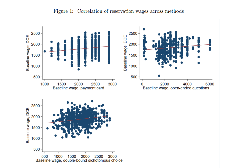
The results in Table 1 showcase that there are large economically and statistically significant differences in reservation wages depending on the method used to estimate them. In Figure 1 we plot the reservation wages estimated from the DCE compared to the reservation wages estimated from each of the three other methods. The figure shows that these are not simply differences in levels: the correlation of reservation wages within person estimated with the DCE and each of the alternative elicitation method is low at around 0.14-0.21. Overall, these results suggests that researchers should carefully consider how the method used to collect reservation wage data could impact their results and analysis. But which of these methods provide the estimates closest to the truth? The next section utilizes estimates from valuing job attributes to make the case that discrete choice experiments provide estimates that are most consistent with reality.
We estimate the value that jobseekers place on different job amenities in Table 2. Column 1 presents the estimates from the open ended questions. This method estimates that individuals would need to be paid approximately 153EGP more per month to accept a job that is a 60 minute commute from home, relative to one that is a 30 minute commute from home. This increases to an additional 304EGP a month for a job that is 120 minutes from home. We find that individuals would be willing to accept a job that pays 301EGP less if that job also offers health insurance, while needing an additional 320EGP to work on Friday, the first day of the weekend in Egypt. Estimates on the value of meals and daycare are smaller and statistically insignificant. Overall the estimates from the open ended questions are not very precisely estimated due to their susceptibility to outliers. In Column 2 we present estimates after winsorizing values at the top and bottom 1%. Doing so decreases our standard errors by a factor of 2 and up to a factor of nearly 4. This leads to results that are more logically consistent: the cost of longer commutes goes up, and the value of health insurance for two people is now larger than for one (both things that didn’t hold without winsorizing). On the other hand we find that free meals and child care are valued as disamenities.7
Column 3 reports the estimates when using the payment card method. These estimates are much more precisely estimated, but this is primarily due to the restrictive nature of the allowable responses. By limiting answers to a small set of choices, this method minimizes outliers and removes some of the natural variation that comes from continuous variables. While smaller standard errors are often attractive, in this case there are several instances where estimates are not logically consistent. For example, commuting 90 minutes requires a larger compensating differential than commuting 120 minutes and the value of health insurance for 1 person is larger than for 2 people. These estimates are not only at odds with the theory of compensating differentials, but also with recent empirical findings (Le Barbanchon et al., 2020).
Column 4 presents estimates using the double-bound dichotomous choice format. This method has fewer inconsistencies relative to the other methods, with the only two surprises being that there is almost no value placed on meals at the workplace and that free daycare is seen as a disamenity, with estimates suggesting that individuals would need to be paid 59 EGP more to take a job that provides that service.
Column 5 provide the estimates from the Discrete Choice Experiment (DCE) elicitation. As described above, we implemented the DCE on the full sample, as we hypothesized that this method would be the most accurate. To make the comparison of the DCE results to the other methods similar in the number of observations, we chose a random third of the sample to analyze in this table. Estimates that utilize all the data we collected are reposed in Column 1 of Table 3.
We find that the DCE provides estimates with standard errors that are close to those of the double bound method. At the same time the estimates are the most consistent with earlier work and our understanding of the labor market. Compensating differentials increase with commute time, the value of health insurance increases when it covers spouses in addition to the employee, and free meals are seen as a valuable amenity that make people want the job more, as is free daycare. Overall, the results from Table 2 suggest that the DCE method provides estimates that are most accurate relative to all other methods.
We complement the experimental analysis with data obtained during a follow-up survey that was carried out in December 2020 (between 1.5 and 2 years after the baseline survey). In this survey, we asked individuals who had found a job since the baseline about its characteristics. We were able to survey 986 individuals (50% of our original sample).8 Thankfully Table A6 shows that attrition is not correlated with the elicitation method assigned at baseline, even though men and married individuals were in general more likely to be found at follow-up. Of the individuals resurveyed, 891 had worked since the time they completed the baseline survey and could thus provide us information about the characteristics of their current or most recent job
We use these data in a regression where we interact each job amenity with a binary variable that takes the value 1 if their most recent job contained that amenity. We contend that these interactions should be either negative or null, indicating that those whose job include a particular amenity were likely to have valued it more at baseline, and when a job includes a disamenity those who “select” into it require a lower differential compensation relative to the average worker. Table 4 presents the results of this analysis. Columns 1 and 2 show once again that using open-ended questions produces inconsistent estimates for some attributes: individuals whose job includes health insurance were willing to pay less for this amenity at baseline than those whose job did not include health insurance. Column 3 presents the estimates from the Payment Card format, showing no significant differences in WTP by presence of each attribute in the current/most recent job except for health insurance. However, the inconsistencies regarding compensation for longer commutes in the main effects persist. Similarly, estimates obtained using the Double Bound Dichotomous Choice format (column 4) show no statistically significant differences for the interaction terms with the exception of the need to work on weekends, where the point estimate is positive and marginally significant. Finally, estimates using the DCE method show the expected results: estimates for the main effects have signs consistent with the idea that individuals will require a compensation for a disamenity and would be willing to forgo part of their wage in exchange for a job amenity. Interaction terms are either negatively signed or statistically indistinguishable from zero. The only exception is health insurance for the worker and their spouse, which estimate is positive but only marginally significant (with a p-value of 0.096). The fact that the DCE results are the only method that provide estimates on all of the job attributes in line with basic economic theory leads us to prefer the DCE method over the others for their accuracy. This is in line with our prior expectations, since discrete choice experiments mimic real world decisions better than the other methods.
We also use the follow up data to assess how well the different methods perform in estimating reservation wages. We regress the originally estimated reservation wages on baseline demographic characteristics including gender, age, education and prior work status. We take the residual of this regression and characterize individuals with a higher residual as “choosy”, i.e. these are people whose reservation wages are higher than we would expect given their characteristics. We then test if those who have high residuals are less likely to have found a suitable job in the time between baseline and our follow up survey.
Figure 2 shows how each method performs on this test. We split individuals into deciles based on the residual in the regression, and then plot the proportion of individuals in each decile who are currently working or have worked at all during the follow up period. We expected the pattern to be downward sloping, with higher deciles having lower work propensities. Across all four methods the relationships between working and the residual are relatively flat. We interpret this as evidence that all methods struggle to predict who will be unemployed in the longer term.
In addition to comparing the estimates across elicitation methods we implemented a few small experiments that allow us to test for consistency within an elicitation method. These experiments allow us to test whether responses depend on the order the questions are presented to the respondents as well as if the range of values provided in the pay-card and double-bound methods affect valuation estimates.
In the first auxiliary experiment, some individuals were assigned a first job offer that does not include health insurance, and the second and third offers added this amenity for themselves and their spouses, respectively. Another group of respondents faced a first job offer that included health insurance for themselves and their spouse, and the following two offers progressively removed the number of people covered by this amenity.
The results are shown in Table B1. We see that the interaction effect for health insurance with the spouse is always statistically different from zero, which indicates that the sequencing of the questions matters. The negative coefficient indicates that individuals value health insurance more when they “lose” this benefit, consistent with loss aversion.
In the second auxiliary experiment we vary the range of options individuals are provided in the payment card and double bound methods. For the payment card method some individuals were shown “low” values (EGP 1000 to EGP 2200 in EGP 200 intervals) and others were shown “high” values (EGP 1400 to EGP 2600 in EGP 200 intervals). Appendix Table B2 presents estimates for the payment card format including interaction terms between each attribute and an indicator for being shown the “low values”. Those shown a card with lower values tend to have an average reservation wage EGP 250/270 lower than those shown the card with higher values. This shows that estimates using the payment card method are sensitive to the values chosen by the researchers.
A final auxiliary experiment changes the value that was added or subtracted to the response given using the double bound method. Appendix Table B3 reports dummy variables for the different values that are added or subtracted from the baseline wage. The estimates from columns 1 & 2 are nearly identical, implying that the results are not sensitive to this parameter.
A major benefit of being able to estimate the value of job attributes is the ability to understand how the value of these attributes differ by job seeker characteristics. Previous studies have shown that men and women have different preferences for attributes such as commute time (Le Barbanchon et al., 2020) and work flexibility (Mas and Pallais, 2017). We are able to expand on this earlier work by considering additional attributes like meals and childcare.
Table 3 presents the estimates of job attribute valuations from the discrete choice experiment for men and women separately. Column 1 includes estimates from using all the data we collected from the pooled sample.9 We have more than twice as many men in our sample as women, so confidence intervals for women tend to be larger.
The results show that men and women have different willingness to pay for some of the attributes we included in our survey. First, men have a 30% higher baseline wage than women. We also find that women require almost twice as much compensation to accept jobs that are further away from their homes relative to men. We also find that women are more sensitive to working on weekends. and value childcare more, although these estimates are not statistically different from each other.
Table A7 considers how valuations differ by gender using the other elicitation methods. While these methods are not well powered, and so most differences are not statistically significant, we compare the point estimates to get some idea of how the methods line up with our understanding of the labor market.
Our results lead to several important implications. First, estimated reservation wages and the valuation of job attributes are sensitive to the method used to elicit them. This is particularly important since the worst performing method to estimate reservation wages (open ended questions) is the method that is most widely used in the literature (Krueger & Mueller, 2016). Scholars and practitioners would be better served using different methods, with discrete choice experiments performing best. While discrete choice experiments may seem more involved, they are also more intuitive to respondents, and only took 40 seconds longer to implement on average in our survey relative to the open ended questions commonly used in the literature.
Our results also speak to how valuation for job attributes differ by individual characteristics. This is directly relevant for efforts that try to increase labor force participation by underrepresented groups. By identifying which job attributes are most highly valued by individuals in those groups policymakers could target those types of amenities through subsidies or direct regulation. For example, women are more sensitive to long commutes, and wefind suggestive evidence that daycare options were more valued by women, who are woefully underrepresented in the Egyptian labor market, where female labor force participation is 23% (ILO, 2016).10 Implementing these types of surveys on a larger and more varied sample can allow for a feasible way to estimates how different groups value different job amenities and provide policymakers with the ability to support particular groups with targeted regulations and subsidies (e.g. by subsidizing daycare, or allowing industries that heavily utilize female employees zoning exceptions to bring them closer to where people live. There is an existing program in Egypt that attempts to do this that translates to “Work near where you live”). These methods could be especially useful in developing country contexts where information frictions abound and knowledge of how different aspects of jobs are valued by different population groups is scarce. Another important way to utilize these results would be for firms to implement this type of measurement procedures with existing or potential employees. This can help firms craft bundles of amenities that are more in line with employee preferences. For example, if employees value certain perks that are less costly for the employer to provide than for the employee to provide for themselves (like meals, or daycare, or a gym, etc) then it may be worthwhile for the employer to begin incorporating those perks into the offer bundle to employees, even if that leads to a decrease in the overall salary provided. Linking these types of data with data on worker productivity could also provide an effective device to bring in the most productive workers (in line with the interview incentives provided in Abebe et al. (2019)).
As with any research endeavor, our study has several limitations to consider. One important limitation is that our follow up survey does not provide bulletproof evidence regarding which of the methods performs best in the real world. While our estimates of how the valuation of job attributes differ across methods, and the DCE provides the estimates most consistent with the previous literature and our understanding of the labor market, this does not mean that it is correct. For example, we used the valuations placed on free meals and free daycare to disqualify measurement strategies that provided estimates that gave negative values to positive amenities. There is a chance that these amenities are seen as indicators of other aspects of the jobs that job seekers try to avoid. For example, maybe working at a place that has free meals is associated with a low prestige set of jobs and the negative valuation is a proxy for the prestige of the job and not the meals itself. We are not able to rule out this possibility. On the other hand, the estimated value of the meals is in line with the market price of meals in this context. Second, our estimates of the differences in the valuation of job attributes by gender are lower powered than we had anticipated. By replicating this analysis with a larger sample researchers would be able to more precisely showcase differences in valuation of job attributes by gender and other characteristics of interest such as education, marital status, etc. We are currently too low powered to properly explore those dimensions. Finally, our sample is comprised of individuals who have selected into working with a particular job matching center. The valuations that we estimate are going to be dependant on those in our sample. Our estimates about the differences between men and women may just be a difference between the men and women who use this job matching center. This issue of external validity is important in any study of a non-representative sample. We compare our sample to a representative survey, which allows us to show that our sample is similar to the general jobseeker population in out context. Nonetheless we cannot rule out that there may be important differences in unobservable characteristics.
Reservation wages and the value placed on non-wage job amenities are important parts of understanding labor market behavior of jobseekers. These parameters can help policymakers generate more effective employment tax and incentive schemes and help employers craft more efficient employee compensation bundles. Identifying which amenities are most valuable to underrepresented groups in the labor market could help policymakers provide targeted subsidies that could encourage greater engagement by those groups. However, estimating the value that workers assign to job characteristics has proven challenging.
We find large differences in the estimates obtained using 4 different elicitation methods. Estimated reservation wages range from 1861 EGP to 2515 EGP. Estimated job amenity values can also differ widely by method. For instance the estimated compensating differential for working on the weekend ranges from EGP 326, or 13% of the baseline wage using open ended questions, to 134 EGP or 6% of the baseline salary using pay-card elicitation.
Overall, estimates from the discrete choice experiment perform best. DCE estimates are most consistent with our understanding of the labor market, basic economic theory, and estimates from other papers in the literature. Future work could benefit from implementing these tests on different samples and with other job attributes. Finding a logistically feasible way to validate the results of these methods with a revealed preference approach using real jobs would be of high value. Validation exercises as in Mas and Pallais (2017) & He et al. (2021) are difficult to implement on a specific sample, whereas the methods outlined in this paper are easier to implement in a variety of contexts. Collecting these data over time for the same set of job seekers would also be useful and could provide information on the dynamics of reservation wages as well as how valuations of different job attributes change over time. This could be valuable even after individuals find a job, as the value placed on certain amenities can change as people’s work experience allow them to learn more about which amenities they value most in a job.
Abebe, G., Caria, S., & Ortiz-Ospina, E. (2019). The selection of talent.
Adamowicz, W., Louviere, J., & Williams, M. (1994). Combining revealed and stated preference methods for valuing environmental amenities. Journal of environmental economics and management, 26(3), 271–292.
Bateman, I. J., Carson, R. T., Day, B., Hanemann, M., Hanley, N., Hett, T., et al. (2002). Economic valuation with stated preference techniques: A manual.
Brown, T. C., Champ, P. A., Bishop, R. C., & McCollum, D. W. (1996). Which response format reveals the truth about donations to a public good? Land Economics, 152–166.
Caliendo, M., Lee, W.-S., & Mahlstedt, R. (2017). The gender wage gap and the role of reservation wages: New evidence for unemployed workers. Journal of Economic Behavior & Organization, 136, 161–173.
Caliendo, M., Tatsiramos, K., & Uhlendorff, A. (2013). Benefit duration, unemployment duration and job match quality: A regression-discontinuity approach. Journal of applied econometrics, 28(4), 604–627.
Cameron, A. C. & Trivedi, P. K. (2005). Microeconometrics: Methods and applications. Cambridge university press.
Cameron, T. A., Poe, G. L., Ethier, R. G., & Schulze, W. D. (2002). Alternative non-market value-elicitation methods: Are the underlying preferences the same? Journal of Environmental Economics and Management, 44(3), 391–425.
Carson, R. T. & Hanemann, W. M. (2005). Contingent valuation. Handbook of environmental economics, 2, 821–936.
Carson, R. T., Mitchell, R. C., Hanemann, M., Kopp, R. J., Presser, S., & Ruud, P. A. (2003). Contingent valuation and lost passive use: Damages from the Exxon Valdez oil spill. Environmental and resource economics, 25(3), 257–286.
Chen, K.-M., Ding, N., List, J. A., & Mogstad, M. (2020). Reservation wages and workers’ valuation of job flexibility: Evidence from a natural field experiment. University of Chicago, Becker Friedman Institute for Economics Working Paper, (2020-124).
Dal Bó, E., Finan, F., & Rossi, M. A. (2013). Strengthening state capabilities: The role of financial incentives in the call to public service. The Quarterly Journal of Economics, 128(3), 1169–1218.
DellaVigna, S., Lindner, A., Reizer, B., & Schmieder, J. F. (2017). Reference-dependent job search: Evidence from Hungary. The Quarterly Journal of Economics, 132(4), 1969–2018.
Diamond, P. A. & Hausman, J. A. (1994). Contingent valuation: Is some number better than no number? Journal of economic perspectives, 8(4), 45–64.
Eriksson, T. & Kristensen, N. (2014). Wages or fringes? Some evidence on trade-offs and sorting. Journal of Labor Economics, 32(4), 899–928.
Faberman, R. J., Mueller, A. I., Şahin, A., & Topa, G. (2017). Job search behavior among the employed and non-employed. National Bureau of Economic Research.
Greene, W. H. & Hensher, D. A. (2003). A latent class model for discrete choice analysis: Contrasts with mixed logit. Transportation Research Part B: Methodological, 37(8), 681–698.
Hall, R. E. & Mueller, A. I. (2018). Wage dispersion and search behavior: The importance of nonwage job values. Journal of Political Economy, 126(4), 1594–1637.
Hanemann, M., Loomis, J., & Kanninen, B. (1991). Statistical efficiency of double-bounded dichotomous choice contingent valuation. American journal of agricultural economics, 73(4), 1255–1263.
Hanley, N., Wright, R. E., & Adamowicz, V. (1998). Using choice experiments to value the environment. Environmental and resource economics, 11(3-4), 413–428.
He, H., Neumark, D., & Weng, Q. (2021). Do workers value flexible jobs? A field experiment. Journal of Labor Economics, 39(3), 709–738.
ILO. (2016). Employment by sex and age – ILO modelled estimates. ILOSTAT. https://ilostat.ilo.org/data.
Koenig, F., Manning, A., & Petrongolo, B. (2016). Reservation wages and the wage flexibility puzzle.
Krueger, A. B. & Mueller, A. I. (2016). A contribution to the empirics of reservation wages. American Economic Journal: Economic Policy, 8(1), 142–79.
Lavetti, K. & Schmutte, I. M. (2018). Estimating compensating wage differentials with endogenous job mobility.
Le Barbanchon, T., Rathelot, R., & Roulet, A. (2019). Unemployment insurance and reservation wages: Evidence from administrative data. Journal of Public Economics, 171, 1–17.
Le Barbanchon, T., Rathelot, R., & Roulet, A. (2020). Gender differences in job search: Trading off commute against wage. Quarterly Journal of Economics.
Maestas, N., Mullen, K. J., Powell, D., Von Wachter, T., & Wenger, J. B. (2018). The value of working conditions in the United States and implications for the structure of wages. National Bureau of Economic Research.
Mas, A. & Pallais, A. (2017). Valuing alternative work arrangements. American Economic Review, 107(12), 3722–59.
McFadden, D. & Train, K. (2000). Mixed MNL models for discrete response. Journal of applied Econometrics, 15(5), 447–470.
Mitchell, R. C. & Carson, R. T. (1981). An experiment in determining willingness to pay for national water quality improvements. Draft report to the US Environmental Protection Agency, Washington, DC.
OAMDI. (2019). Harmonized labor force surveys (HLFS). http://erf.org.eg/data-portal/.
Revelt, D. & Train, K. (1998). Mixed logit with repeated choices: Households’ choices of appliance efficiency level. Review of economics and statistics, 80(4), 647–657.
Rosen, S. (1986). The theory of equalizing differences. Handbook of labor economics, 1, 641–692.
Rowe, R. D., Schulze, W. D., & Breffle, W. S. (1996). A test for payment card biases. Journal of environmental Economics and management, 31(2), 178–185.
Stern, S. (2004). Do scientists pay to be scientists? Management science, 50(6), 835–853.
Tourangeau, R., Rips, L. J., & Rasinski, K. (2000). The psychology of survey response. Cambridge University Press.
Welsh, M. P. & Poe, G. L. (1998). Elicitation effects in contingent valuation: Comparisons to a multiple bounded discrete choice approach. Journal of environmental economics and management, 36(2), 170–185.
Wiswall, M. & Zafar, B. (2017). Preference for the workplace, investment in human capital, and gender. The Quarterly Journal of Economics, 133(1), 457–507.
Figure 1: Correlation of reservation wages across methods
Note: The Figure shows the reservation wages estimated for each individual from the discrete choice experiment and the alternative elicitation method to which they were assigned. These reservation wages correspond to the minimum wage at which an individual would accept a job that is 30 minutes away from their home and has none of the attributes included in our survey. The correlation coefficients between the reservation wages estimated from the discrete choice experiment and the other elicitation methods are 0.14 in the case of the open-ended questions and 0.21 in the case of the payment card and double-bound dichotomous choice questions.
Figure 2: Probability of ever being employed by decile of reservation wage’s residual
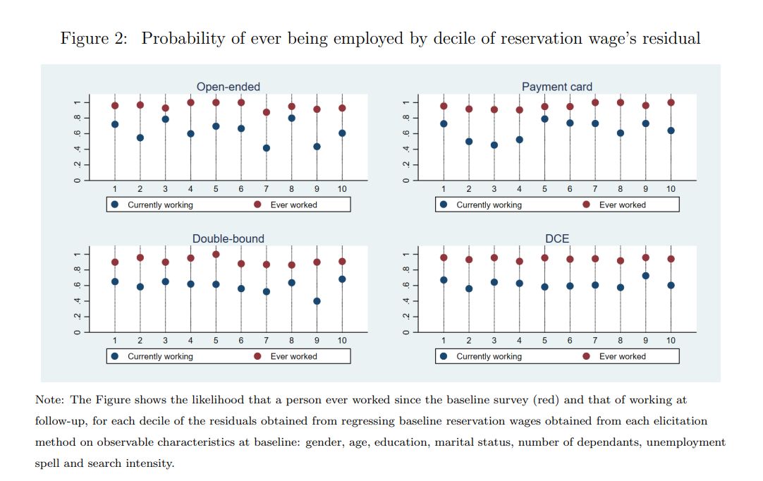
Note: The Figure shows the likelihood that a person ever worked since the baseline survey (red) and that of working at follow-up, for each decile of the residuals obtained from regressing baseline reservation wages obtained from each elicitation method on observable characteristics at baseline: gender, age, education, marital status, number of dependants, unemployment spell and search intensity. Larger residuals correspond to higher reservation wages than we would predict based on the individual’s observable characteristics.
Table 1: Difference between wages at baseline across formats
Panel A: Estimated Reservation Wages
| (1) Open Ended | (2) Open Ended Winsorized | (3) Payment Card | (4) Double Bound | (5) Discrete Choice Experiment | |
|---|---|---|---|---|---|
| Reservation wage for baseline job | 2711 | 2515 | 2238 | 2045 | 1778 |
| (157.77) | (38.11) | (20.16) | (29.58) | (42.21) | |
| Observations | 4620 | 4620 | 4704 | 4634 | 9975 |
| Number of Individuals | 660 | 660 | 672 | 662 | 665 |
Panel B: P-Values for Pair-wise Comparisons of Reservation Wages
| Payment Card | Double Bound | Discrete Choice Experiment | |
|---|---|---|---|
| Open Ended | 0.003 | 0.000 | 0.000 |
| Payment Card | 0.000 | 0.000 | |
| Double Bound | 0.000 |
Notes: Panel A reports estimated reservation wages using each method, but chooses one third of the Discrete Choice Experiment sample to keep the number of individual respondents similar. Standard errors clustered at the individual level in parentheses. Panel B reports the p-value of the test that the wage at baseline is equal between the elicitation format depicted in the row title and the elicitation format in the column title.
Table 2: Estimates of willingness to pay for job attributes according to each elicitation format
| Open ended | Open ended winsorized | Payment Card | Double Bound | Discrete choice experiment | |
|---|---|---|---|---|---|
| (1) | (2) | (3) | (4) | (5) | |
| Commute time (60 Minutes) | 152.79 | 182.59*** | 37.75 | 184.15*** | 65.65*** |
| (123.20) | (55.53) | (40.00) | (51.63) | (22.56) | |
| Commute time (90 Minutes) | 148.58 | 273.37*** | 159.38*** | 190.25*** | 155.32*** |
| (105.51) | (59.88) | (45.20) | (52.95) | (49.11) | |
| Commute time (120 Minutes) | 303.77*** | 407.58*** | 67.63* | 203.27*** | 327.29*** |
| (107.82) | (62.93) | (35.67) | (53.36) | (36.34) | |
| Health insurance (self) | -301.43*** | -126.58*** | -145.45*** | -132.95*** | -76.70** |
| (105.16) | (29.14) | (19.07) | (35.64) | (20.69) | |
| Health insurance (self & spouse) | -221.99** | -117.02** | -91.24*** | -231.73*** | -156.52*** |
| (86.21) | (45.66) | (30.37) | (22.70) | (29.61) | |
| Need to work on weekends | 320.68*** | 325.41*** | 134.42*** | 233.71*** | 165.39*** |
| (109.39) | (28.20) | (17.02) | (34.32) | (22.00) | |
| Meals provided at workplace | 14.46 | 83.82*** | -18.12 | -4.6 | -63.31** |
| (87.46) | (24.68) | (15.34) | (33.32) | (19.61) | |
| Daycare provided at workplace | -45.10 | 81.83*** | -10.59 | 58.93* | 2.1 |
| (77.37) | (24.66) | (17.20) | (33.47) | (14.45) | |
| Observations | 4620 | 4620 | 4704 | 4634 | 9975 |
| Number of individuals | 660 | 660 | 672 | 662 | 665 |
Notes: Each column reports the willingness to pay for each job
attribute obtained from the different elicitation methods. Open-ended
estimates were obtained by regressing the stated wage on indicators for
each of the characteristics specified. Payment card estimates were
obtained by maximum likelihood where the dependent variable is the
interval between the value chosen and the closest value available below
the one chosen, using a model where all characteristics are interacted
with a dummy that takes value 1 if the payment card shows a range of
lower values. Double bound estimates were obtained by maximum likelihood
using the intervals provided by the Yes/No answers to each job offer
given by the respondent. Discrete choice experiment correspond to a
random sample of one third of respondents to match the sample size to
those of other elicitation methods. Estimates were obtained using a
mixed logit model in the willingness to pay space estimated by maximum
likelihood. Estimates for the winsorized open-ended format obtained by
winsorizing at the top and bottom 1% of responses. Standard errors
clustered at the individual level between parenthesis.
*** p<0.01, ** p<0.05, *p<0.1
Table 3: Discrete choice experiment estimates by gender
| (1) Pooled Sample | (2) Men | (3) Women | (4) P-value of Difference | |
|---|---|---|---|---|
| Commute time (60 Minutes) | 98.31*** | 75.69*** | 166.31*** | 0.06 |
| (21.53) | (21.12) | (45.10) | ||
| Commute time (90 Minutes) | 183.20*** | 158.53*** | 266.83*** | 0.30 |
| (23.27) | (33.97) | (87.30) | ||
| Commute time (120 Minutes) | 259.76*** | 251.60*** | 439.21*** | 0.08 |
| (25.90) | (19.56) | (107.35) | ||
| Health insurance (self) | −55.44*** | −65.38*** | −27.4 | 0.32 |
| (13.42) | (17.77) | (34.99) | ||
| Health insurance (self & spouse) | −150.59*** | −154.62*** | −120.37** | 0.56 |
| (14.97) | (17.88) | (55.51) | ||
| Need to work on weekends | 118.78*** | 118.53*** | 172.93*** | 0.26 |
| (16.38) | (20.42) | (38.89) | ||
| Meals provided at workplace | −84.43*** | −61.63*** | −95.8 | 0.64 |
| (9.90) | (22.22) | (73.84) | ||
| Daycare provided at workplace | −41.78*** | −12.7 | −114.8 | 0.46 |
| (11.22) | (10.63) | (136.74) | ||
| Reservation wage at baseline | 1831 | 1919 | 1581 | 0.01 |
| Observations | 29940 | 21075 | 8865 | |
| Number of Individuals | 1996 | 1405 | 591 |
Notes: Column 1 shows the estimates of willingness to pay for different job attributes obtained from the discrete choice experiment on the full sample of survey respondents. Columns 2 and 3 present the results for men and women separately, and column 4 shows the p-value of the difference in valuation for each attribute across gender. Reservation wage at baseline corresponds to average salary when the job is 30 minutes away from the respondent’s home and no other attribute is included. Units are in EGP. 1 USD ≈ 16 EGP. Standard errors clustered at the individual level between parentheses. *** p<0.01, ** p<0.05, * p<0.1
Table 4: Willingness to pay for job attributes across elicitation formats using follow-up information
| Open ended | Open ended winsorized | Payment Card | Double Bound | Discrete choice experiment | |
|---|---|---|---|---|---|
| (1) | (2) | (3) | (4) | (5) | |
| Commute time (60 Minutes) | 57.61 | 244.84*** | -62.66 | 142.5 | 88.16* |
| (122.09) | (91.67) | (60.60) | (96.97) | (49.97) | |
| Commute time (90 Minutes) | 41.93 | 264.87** | 208.08*** | 247.53*** | 191.90*** |
| (214.78) | (105.48) | (73.71) | (84.44) | (30.90) | |
| Commute time (120 Minutes) | 231.15 | 450.27*** | 102.57* | 235.42*** | 297.57*** |
| (197.71) | (94.80) | (55.23) | (81.40) | (54.60) | |
| Health insurance (self) | -522.72** | -193.42*** | -154.40*** | -161.33** | -45.48** |
| (244.79) | (61.03) | (37.72) | (62.96) | (19.57) | |
| Health insurance (self & spouse) | -303.08* | -144.66** | -112.20** | -334.26*** | -176.94*** |
| (156.84) | (65.34) | (41.04) | (35.93) | (47.98) | |
| Need to work on weekends | 309.65 | 392.87*** | 156.19*** | 218.26*** | 128.88** |
| (259.99) | (64.14) | (43.37) | (64.39) | (58.08) | |
| Meals provided at workplace | -83.15 | 99.38** | -7.08 | 55.5 | -70.96*** |
| (157.72) | (43.30) | (22.15) | (53.97) | (25.88) | |
| Daycare provided at workplace | -143.24 | 92.91** | 6.77 | 101.53* | -64.16*** |
| (159.36) | (37.54) | (25.91) | (52.50) | (20.40) | |
| Commute time (60 Minutes) × Current /last job | -149.60 | -68.37 | 84.96 | 163.1 | -61.90 |
| (190.86) | (153.11) | (91.89) | (173.69) | (90.86) | |
| Commute time (90 Minutes) × Current /last job | -389.55 | -363.88 | -174.62 | 2989.6 | -134.48*** |
| (345.76) | (352.21) | (199.32) | (10363.53) | (38.15) | |
| Commute time (120 Minutes) × Current /last job | -1143.90*** | -1193.61*** | 102.90 | -359.0 | -465.90*** |
| (142.74) | (114.55) | (257.18) | (488.07) | (85.46) | |
| Health insurance (self) × Current /last job | 314.03** | 226.85** | -9.69 | -46.3 | -53.57 |
| (142.21) | (107.98) | (51.32) | (90.78) | (51.89) | |
| Health insurance (self & spouse) × Current /last job | 1668.98*** | 1726.51*** | -246.82*** | -31.7 | 126.85* |
| (569.09) | (519.16) | (54.69) | (184.17) | (76.11) | |
| Need to work on weekends × Current /last job | -245.07 | -120.45 | -45.26 | 178.60* | 43.04 |
| (220.44) | (106.84) | (53.51) | (92.20) | (66.71) | |
| Meals provided at workplace × Current /last job | 654.72 | 77.25 | 60.14 | -51.0 | -49.83 |
| (750.97) | (177.54) | (74.80) | (131.67) | (62.45) | |
| Daycare provided at workplace × Current /last job | -238.22 | -199.35 | 0.00 | 15.4 | -201.59*** |
| (401.76) | (421.16) | . | (289.00) | (62.66) | |
| Reservation wage at baseline | 3001 | 2583 | 2285 | 2062 | 1924 |
| Observations | 2156 | 2156 | 2114 | 1960 | 40095 |
| Number of Individuals | 308 | 308 | 302 | 280 | 891 |
Notes: Each column reports the willingness to pay for each job attribute obtained from the different elicitation methods at baseline, including interactions between the attribute and whether the respondent’s most recent job includes that attribute when re-interviewed. Open-ended estimates were obtained by regressing the stated wage (Column 1) and the wage winsorized at the top and bottom 1% (Column 2) on indicators for each of the characteristics specified. Payment card estimates were obtained by maximum likelihood where the dependent variable is the interval between the value chosen and the closest value available below the one chosen, and includes interactions between each characteristic and a dummy that takes value 1 if the payment card shows a range of lower values. Double bound estimates were obtained by maximum likelihood using the intervals provided by the Yes/No answers to each job offer given by the respondent. Discrete choice experiment estimates were obtained using a mixed logit model in the willingness to pay space estimated by maximum likelihood. Reservation wage at baseline corresponds to average salary when the job is 30 minutes away from the respondent’s home and no other attribute is included. Standard errors clustered at the individual level between parenthesis. *** p<0.01, ** p<0.05, *p<0.1
Figure A1: Example of open-ended question asked to respondents
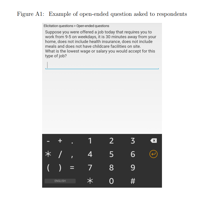
Figure A2: Example of payment card question asked to respondents
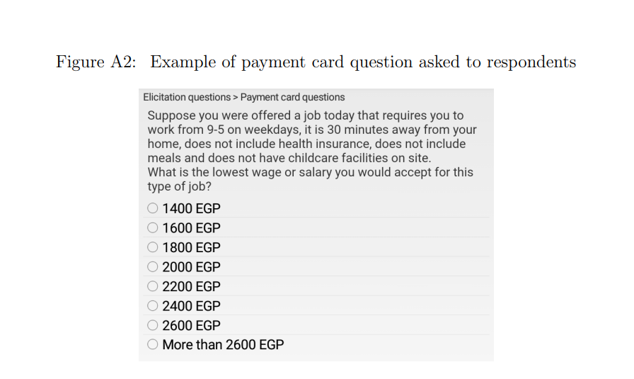
Figure A3: Example of double-bound dichotomous choice question asked to respondents
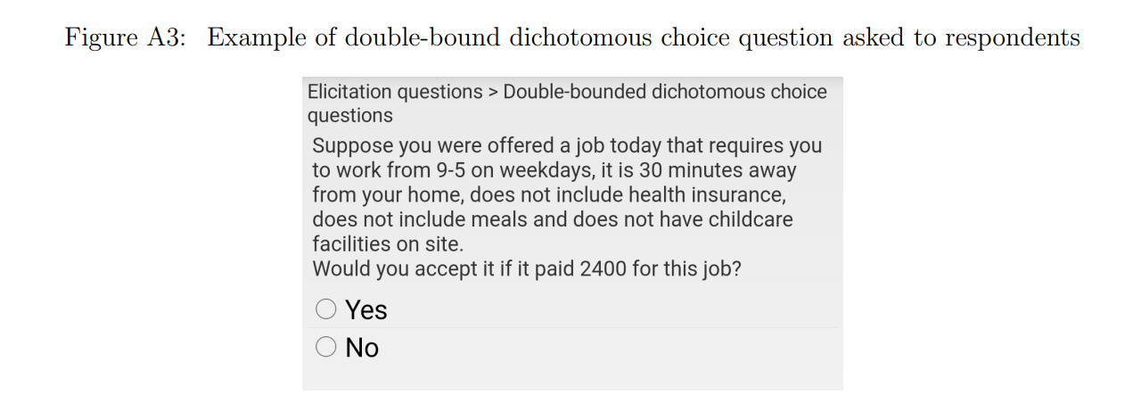
Figure A4: Example of discrete choice question asked to respondents
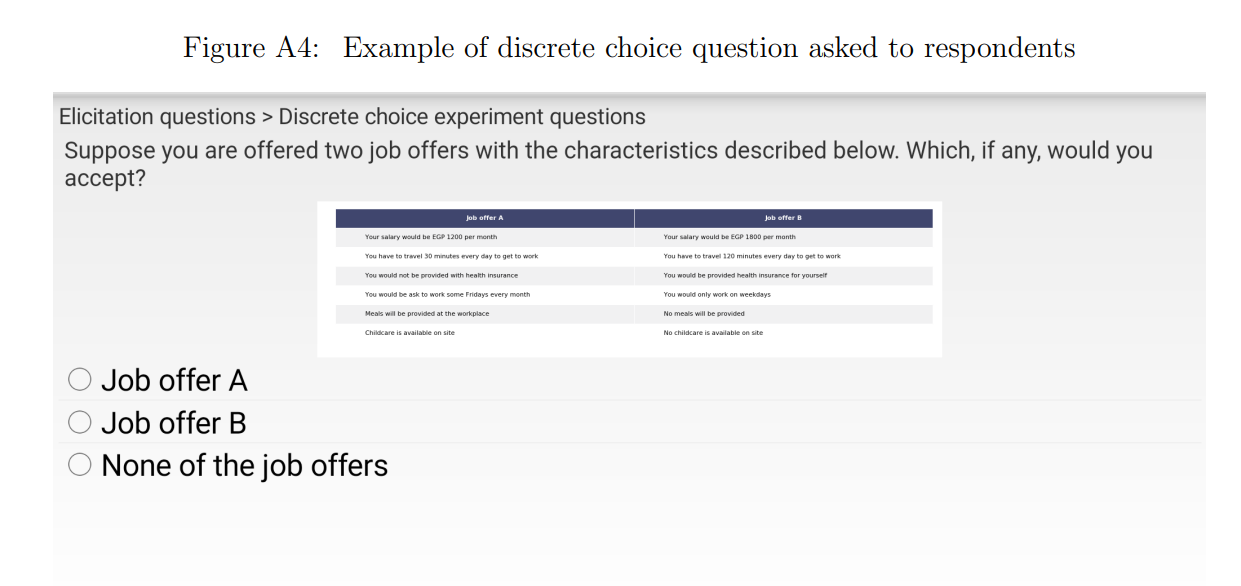
Table A1: Job attributes included in the survey and their values
| Attribute | Levels |
|---|---|
| Commute time (one-way) | 30 minutes |
| 60 minutes | |
| 90 minutes | |
| 120 minutes | |
| Included health insurance | No |
| For the worker | |
| For the worker and spouse | |
| Need to work on weekends | No |
| Some weekends | |
| Meals provided | No |
| Yes | |
| On-site daycare | No |
| Yes |
Note: The table shows the different job attributes that could vary in the hypothetical job offers presented to a respondent. Except in the case of the Discrete Choice Experiment, only one job attribute was varied at a time with each offer shown.
Table A2: Summary statistics of survey respondents and comparison with 2017 Labor Force Survey
| All | Men | Women | |||||||
|---|---|---|---|---|---|---|---|---|---|
| Mean | SD | N | Mean | SD | N | Mean | SD | N | |
| Age | 26.64 | 6.19 | 1996 | 27.27 | 6.28 | 1405 | 25.15 | 5.73 | 591 |
| Share male | 0.70 | 0.46 | 1996 | ||||||
| Share married | 0.29 | 0.46 | 1637 | 0.30 | 0.46 | 1159 | 0.28 | 0.45 | 478 |
| Number of dependents | 0.87 | 1.20 | 1637 | 0.91 | 1.26 | 1159 | 0.78 | 1.04 | 478 |
| Years of education | 12.83 | 4.00 | 1637 | 12.78 | 3.93 | 1159 | 12.94 | 4.18 | 478 |
| Unemployment spell (months) | 8.27 | 16.54 | 1628 | 8.00 | 16.55 | 1143 | 8.92 | 16.51 | 485 |
| Hours spent last week looking for a job | 20.41 | 20.32 | 1679 | 21.67 | 20.80 | 1175 | 17.47 | 18.86 | 504 |
| Hours spent on average looking for a job | 14.31 | 15.86 | 1679 | 15.70 | 16.75 | 1175 | 11.07 | 13.01 | 504 |
| Number of methods used to look for a job | 1.70 | 1.56 | 1996 | 1.69 | 1.60 | 1405 | 1.72 | 1.47 | 591 |
| All | Men | Women | |||||||
|---|---|---|---|---|---|---|---|---|---|
| Mean | SD | N | Mean | SD | N | Mean | SD | N | |
| Age | 25.62 | 6.32 | 8826 | 24.71 | 6.27 | 4661 | 26.66 | 6.23 | 4165 |
| Share male | 0.53 | 0.50 | 8826 | ||||||
| Share married | 0.24 | 0.43 | 8826 | 0.10 | 0.30 | 4661 | 0.40 | 0.49 | 4165 |
| Years of education | 12.47 | 3.82 | 8826 | 11.79 | 4.19 | 4661 | 13.23 | 3.17 | 4165 |
| Unemployment spell (months) | 32.98 | 35.78 | 8826 | 24.08 | 25.44 | 4661 | 43.14 | 42.55 | 4165 |
| Number of methods used to look for a job | 2.28 | 1.40 | 8826 | 2.37 | 1.44 | 4661 | 2.18 | 1.35 | 4165 |
Notes: Panel A shows the mean and standard deviation for demographic characteristics and job search behavior of our survey respondents. Sample size for each characteristic vary depending on our ability to match data from our respondents to that collected by our partner NGO. Panel B presents the corresponding demographic characteristics and search behavior (if available) according to unemployed individuals in the 2017 Labor Force Survey. Hours spent looking for a job and unemployment spell variables winsorized at the bottom and top 5%.
Table A3: Sample characteristics and baseline balance
| (1) Mean for Open-Ended | (2) Assigned to Payment Card | (3) Assigned to Double-Bound | |
|---|---|---|---|
| Age | 26.642 | −0.329 (0.339) | 0.337 (0.340) |
| Share male | 0.722 | −0.023 (0.025) | −0.032 (0.025) |
| Share married | 0.311 | −0.035 (0.028) | −0.018 (0.028) |
| Number of dependents | 0.866 | −0.052 (0.073) | 0.070 (0.073) |
| Years of education | 12.884 | 0.045 (0.242) | −0.214 (0.243) |
| Unemployment spell (months) | 9.071 | −1.650 (1.000) | −0.747 (1.004) |
| Hours spent last week looking for job | 21.355 | −1.210 (1.211) | −1.648 (1.216) |
| Hours spent on average looking for job | 14.590 | −0.888 (0.945) | 0.053 (0.949) |
| Number of methods used | 1.749 | −0.102 (0.086) | −0.047 (0.086) |
| P-value of joint test | 0.429 | 0.389 | |
| Observations | 660 | 672 | 662 |
Notes: Each row presents the mean of the covariate for the individuals assigned to the open-ended formats and the coefficients of a regression of the covariate on indicators that take the value of one if the individual was assigned to the payment card (Column 2) or double-bound dichotomous choice elicitation format (Column 3). Standard errors between parentheses. *** p<0.01, ** p<0.05, * p<0.1
Table A4: List of questions by elicitation method
The following seven hypothetical job offers were presented to participants. Sections in bold show the job attribute that differs from the baseline job described.
Suppose you were offered a job today that requires you to work from 9–5 on weekdays, it is 30 minutes away from your home, does not include health insurance, does not include meals and does not have childcare facilities on site. What is the lowest wage or salary you would accept for this type of job?
Suppose you were offered a job today that requires you to work from 9–5 on weekdays, it is 30 minutes away from your home, it offers health insurance for you, but does not include meals or daycare on site. What is the lowest wage or salary you would accept for this type of job?
Suppose you were offered a job today that requires you to work from 9–5 on weekdays, it is 30 minutes away from your home, it offers health insurance for you and your spouse, but does not include meals or childcare facilities on site. What is the lowest wage or salary you would accept for this type of job?
Suppose you were offered a job today that requires you to work from 9–5 on weekdays, it is X minutes away from your home, does not include health insurance, does not include meals and does not have childcare facilities on site. What is the lowest wage or salary you would accept for this type of job?
Suppose you were offered a job today that requires you to work from 9–5 on weekdays and requires you to work on Friday instead of a weekday twice a month, it is 30 minutes away from your home, does not include health insurance, does not include meals and does not have childcare facilities on site. What is the lowest wage or salary you would accept for this type of job?
Suppose you were offered a job today that requires you to work from 9–5 on weekdays, it is 30 minutes away from your home, does not include health insurance, includes meals at work, and does not have childcare facilities on site. What is the lowest wage or salary you would accept for this type of job?
Suppose you were offered a job today that requires you to work from 9–5 on weekdays, it is 30 minutes away from your home, does not include health insurance, does not include meals, but has on-site childcare facilities. What is the lowest wage or salary you would accept for this type of job?
Note: In the case of open ended questions, the respondent enters a value to answer each question. For payment card questions, the respondent is asked to choose a value from a list showed below each question. In the case of dichotomous choice questions, the question is replaced by “Would you accept it if it paid $Z for this job?”, where Z is a salary chosen at random. The value of X in question 4 is one of either 60, 90 or 120 minutes.
Table A5: Estimates of open-ended elicitation method with winsorized values
| Cutoff | (1) 0% | (2) 1% | (3) 2% | (4) 5% |
|---|---|---|---|---|
| Commute time (60 Minutes) | 152.79 | 182.59*** | 179.72*** | 171.92*** |
| (123.20) | (55.53) | (52.56) | (41.50) | |
| Commute time (90 Minutes) | 148.58 | 273.37*** | 272.55*** | 241.82*** |
| (105.51) | (59.88) | (57.31) | (46.25) | |
| Commute time (120 Minutes) | 303.77*** | 407.58*** | 379.32*** | 307.46*** |
| (107.82) | (62.93) | (57.58) | (45.58) | |
| Health insurance (self) | −301.43*** | −126.58*** | −117.68*** | −95.06*** |
| (105.16) | (29.14) | (27.84) | (20.91) | |
| Health insurance (self & spouse) | −221.99** | −117.02** | −108.38** | −88.68** |
| (86.21) | (45.66) | (43.26) | (34.70) | |
| Need to work on weekends | 320.68*** | 325.41*** | 315.77*** | 279.73*** |
| (109.39) | (28.20) | (26.58) | (19.30) | |
| Meals provided at workplace | 14.46 | 83.82*** | 81.83*** | 73.21*** |
| (87.46) | (24.68) | (23.54) | (16.90) | |
| Daycare provided at workplace | −45.10 | 81.83*** | 83.62*** | 75.38*** |
| (77.37) | (24.66) | (23.82) | (17.86) | |
| P-value of equality of coefficients | 0.000 | |||
| Wage at baseline (EGP) | 2711 | 2517 | 2506 | 2520 |
| Observations | 4620 | 4620 | 4620 | 4620 |
| Number of Individuals | 660 | 660 | 660 | 660 |
Notes: The table shows estimates from the open ended elicitation format when responses are unwinsorized (column 1), and winsorized at the 1, 2 and 5% of the bottom and top of the distribution of responses (columns 2 to 4). Baseline wage corresponds to average salary when the job is 30 minutes away from the respondent’s home and no other attribute is included. Units are in EGP. 1 USD ≈ 16 EGP. Standard errors clustered at the individual level between parentheses. *** p<0.01, ** p<0.05, * p<0.1
Table A6: Baseline determinants of the probability of being found at follow-up
| Dependent variable: Found at follow-up | (1) Open Ended | (2) Payment Card | (3) Double Bound |
|---|---|---|---|
| Male indicator | 0.137** (0.055) | 0.023 (0.078) | −0.082 (0.077) |
| Age | 0.001 (0.005) | −0.001 (0.007) | −0.001 (0.007) |
| Reservation wage estimated from DCE | −0.076 (0.070) | 0.008 (0.104) | 0.153 (0.102) |
| Married indicator | 0.040** (0.018) | −0.025 (0.025) | −0.039 (0.025) |
| Education level | 0.036 (0.029) | −0.002 (0.043) | −0.046 (0.039) |
| Number of dependants | 0.001 (0.001) | 0.000 (0.002) | 0.001 (0.002) |
| Job search spell, in months | −0.000 (0.000) | 0.000 (0.000) | 0.000 (0.000) |
| Constant | 0.216 (0.213) | 0.105 (0.303) | 0.053 (0.303) |
| P-value of H0: No differential attrition | 0.992 | 0.397 | |
| Observations | 1326 | 1326 | 1326 |
Notes: Each column presents the estimates from the interaction of each observable characteristic with an indicator that takes the value of one if the individual was assigned to the corresponding elicitation method at baseline. The base group corresponds to individuals assigned to the open-ended elicitation method. The dependent variable is an indicator that takes the value of one if the person was found at follow-up. Standard errors clustered at the individual level between parentheses. *** p<0.01, ** p<0.05, * p<0.1
Table A7: Treatment effect heterogeneity by gender across elicitation methods
| Open Ended | Pay Card | Double Bound | |||||||
|---|---|---|---|---|---|---|---|---|---|
| Men | Women | P-value of difference | Men | Women | P-value of difference | Men | Women | P-value of difference | |
| (1) | (2) | (3) | (4) | (5) | (6) | (7) | (8) | (9) | |
| Commute time (60 Minutes) | 171.44*** | 184.47* | 0.92 | 77.36** | -24.56 | 0.07 | 183.19*** | 177.00** | 0.96 |
| (64.12) | (103.19) | (31.05) | (46.78) | (62.45) | (90.02) | ||||
| Commute time (90 Minutes) | 295.99*** | 260.77*** | 0.77 | 120.19*** | 157.33*** | 0.53 | 203.33*** | 195.85** | 0.95 |
| (74.01) | (94.68) | (35.22) | (47.11) | (65.96) | (87.22) | ||||
| Commute time (120 Minutes) | 448.24*** | 291.81*** | 0.23 | 70.96** | 113.27** | 0.49 | 178.89*** | 234.65** | 0.63 |
| (74.78) | (105.69) | (28.99) | (53.67) | (63.47) | (95.36) | ||||
| Health insurance (self) | -120.72*** | -138.64*** | 0.76 | -113.37*** | -82.66*** | 0.24 | -95.34** | -204.23*** | 0.15 |
| (36.39) | (44.56) | (15.55) | (21.28) | (43.37) | (61.68) | ||||
| Health insurance (self & spouse) | -110.30** | -128.05 | 0.85 | -78.02*** | -44.94 | 0.44 | -246.32*** | -201.49*** | 0.35 |
| (54.40) | (77.81) | (23.50) | (35.91) | (27.37) | (39.32) | ||||
| Need to work on weekends | 304.35*** | 379.30*** | 0.22 | 116.97*** | 133.08*** | 0.55 | 184.59*** | 331.78*** | 0.04 |
| (34.40) | (49.62) | (13.70) | (22.99) | (41.34) | (59.70) | ||||
| Meals provided at workplace | 83.68*** | 82.73** | 0.98 | 14.6 | 36.85* | 0.36 | -9.4 | 4.91 | 0.84 |
| (31.63) | (36.65) | (13.66) | (19.87) | (40.15) | (58.33) | ||||
| Daycare provided at workplace | 79.32** | 86.92** | 0.87 | -11.4 | 21.29 | 0.19 | 56.1 | 68.14 | 0.87 |
| (31.87) | (35.20) | (14.50) | (20.30) | (40.51) | (58.10) | ||||
| Lower card values | -228.89*** | -147.39*** | 0.17 | ||||||
| (33.87) | (49.44) | ||||||||
| Wage at baseline | 2637 | 2200 | 2342 | 1988 | 2144 | 1839 | |||
| Observations | 3332 | 1288 | 3290 | 1414 | 3199 | 1435 | |||
| Number of Individuals | 476 | 184 | 470 | 202 | 457 | 205 |
Notes: The table shows estimates of the value for each job
characteristic by elicitation method used, for men and women separately.
Open-ended estimates correspond to estimates of the winsorized sample at
the top 1%. Payment card estimates correspond to the specification in
which each attribute is interacted with a dummy that takes value 1 if
the payment card shows a range of lower values. Baseline wage
corresponds to average salary when the job is 30 minutes away from the
respondent’s home and no other attribute is included. Standard errors
clustered at the individual level between parenthesis.
*** p<0.01, ** p<0.05, *p<0.1
In this appendix we present the results of auxiliary experiments we implemented to test the consistency of some elicitation methods used. Table B1 presents estimates of the willingness to pay for health insurance for the job seeker and their spouse for each estimation method and depending on the order in which this job amenity was show to the survey respondents. The reference group was first shown an offer with no health insurance, then an offer with health insurance for themselves and finally a job with health insurance for them and their spouse, while the “treatment” group received these job offers in reverse order. Table B2 presents estimates for the values of different job attributes among individuals assigned to the payment card format for different estimation methods. Column 1 replicates the results from Table 2, showing the maximum likelihood estimates of from the payment card elicitation including an interaction between each attribute and an indicator that takes value 1 when the distribution of options shown to respondents is shifted to the left. Columns 2 and 3 replicate the model of column 1 by OLS when the dependent variable is the value chosen by the individual and the midpoint between the wage chosen and the next lowest value. Table B3 presents estimates for the values of each job attribute among individuals assigned to the double-bound dichotomous choice format. In column 1 the model we estimate includes only the job attributes included in the jobs presented to our survey participants. In column 2, which corresponds to the results presented in Table 2, we include indicators for the magnitude of the difference between the first offer and the second offer we show respondents for each of the jobs. Respondents were assigned to a different magnitude of wage change within this elicitation method. Columns 3-7 presents the results of the model in column 1 for each of the wage difference groups separately.
Table B1: Sensitivity of Responses Based on Randomized First Question in Series
| (1) Open Ended | (2) Payment Card | (3) Double Bound | |
|---|---|---|---|
| Health insurance (self) | −219.08*** (68.77) | −142.64*** (17.59) | −125.50** (53.34) |
| Health insurance (self & spouse) | −176.97* (93.61) | −74.74*** (19.36) | −374.30*** (51.93) |
| Health Insurance (self) × Treatment | −168.99 (283.99) | 7.81 (17.38) | −95.13 (75.30) |
| Health Insurance (self & spouse) × Treatment | −103.56 (317.11) | −13.85 (19.41) | 134.70* (74.02) |
| P-value of no effect for interaction terms | 0.653 | 0.560 | 0.006 |
| Observations | 1980 | 2016 | 1986 |
| Number of Individuals | 660 | 672 | 662 |
Notes: The table shows estimates from the open ended, pay card and double bound dichotomous choice depending on whether the baseline (first) job shown includes health insurance for the respondent and their spouse. Standard errors clustered at the individual level between parentheses. *** p<0.01, ** p<0.05, * p<0.1
Table B2: Comparison of estimates for Payment card format
| (1) Interval | (2) Chosen Value | (3) Midpoint | |
|---|---|---|---|
| Commute time (60 Minutes) | 37.75 (40.00) | 14.85 (34.04) | 39.33 (37.51) |
| Commute time (90 Minutes) | 159.38*** (45.20) | 117.25*** (35.00) | 145.33*** (40.77) |
| Commute time (120 Minutes) | 67.63* (35.67) | 47.24 (30.28) | 55.23 (35.41) |
| Health insurance (self) | −145.45*** (19.07) | −137.95*** (16.67) | −142.72*** (19.02) |
| Health insurance (self & spouse) | −91.24*** (30.37) | −77.06*** (26.03) | −89.52*** (29.74) |
| Need to work on Friday | 134.42*** (17.02) | 116.15*** (14.58) | 132.10*** (17.60) |
| Meals provided at workplace | −18.12 (15.34) | −31.23** (13.58) | −24.29 (15.69) |
| Daycare provided at workplace | −10.59 (17.20) | −23.38 (15.20) | −10.34 (17.36) |
| Lower card values | −255.79*** (38.35) | −273.37*** (31.83) | −256.15*** (36.44) |
| 60-Min commute × Low card values | 7.20 (55.32) | 19.51 (45.47) | 1.31 (50.34) |
| 90-Min commute × Low card values | −63.95 (59.19) | −44.85 (45.40) | −64.02 (52.42) |
| 120-Min commute × Low card values | 73.21 (55.08) | 54.12 (42.07) | 60.79 (49.42) |
| Health insurance (self) × Lower card values | 85.19*** (26.03) | 91.35*** (21.53) | 88.16*** (24.59) |
| Health insurance (self & spouse) × Lower card values | 45.29 (41.92) | 44.23 (34.35) | 49.90 (39.14) |
| Need to work on Friday × Lower card values | −21.01 (23.86) | −32.10* (19.20) | −33.56 (22.58) |
| Meals × Lower card values | 86.78*** (22.54) | 84.80*** (18.57) | 83.81*** (21.50) |
| Daycare × Lower card values | 21.94 (23.71) | 32.13 (20.17) | 19.25 (23.17) |
| Wage at baseline | 2238 | 2291 | 2215 |
| P-value of no effect for interaction terms | 0.000 | 0.000 | 0.000 |
| Observations | 4704 | 4704 | 4704 |
| Number of Individuals | 672 | 672 | 672 |
Notes: Column 1 shows the estimates for each attribute from the payment card elicitation using an interval regression. Column 2 uses the maximum value of the range, while column 3 uses the midpoint of the range. Units are in EGP. 1 USD ≈ 16 EGP. Standard errors clustered at the individual level between parentheses. *** p<0.01, ** p<0.05, * p<0.1
Table B3: Comparison of estimates for the double-bound dichotomous choice format
| (1) Pooled sample | (2) Pooled sample | |
|---|---|---|
| Commute time (60 Minutes) | 182.14*** (51.65) | 184.15*** (51.63) |
| Commute time (90 Minutes) | 191.17*** (52.95) | 190.25*** (52.95) |
| Commute time (120 Minutes) | 203.00*** (53.35) | 203.27*** (53.36) |
| Health insurance (self) | −133.53*** (35.64) | −132.95*** (35.64) |
| Health insurance (self & spouse) | −232.40*** (22.67) | −231.73*** (22.70) |
| Need to work on weekends | 233.32*** (34.33) | 233.71*** (34.32) |
| Meals provided at workplace | −4.3 (33.34) | −4.62 (33.32) |
| Daycare provided at workplace | 59.22* (33.48) | 58.93* (33.47) |
| Wage changes of 200 EGP | 43.28 (33.81) | |
| Wage changes of 300 EGP | 62.08* (34.51) | |
| Wage changes of 400 EGP | 8.37 (34.60) | |
| Wage changes of 500 EGP | −28.31 (33.90) | |
| Reservation wage at baseline | 2045 | 1985 |
| Observations | 4634 | 4634 |
| Number of Individuals | 662 | 662 |
Notes: Column 1 shows the estimates for each attribute using the double bound method without controlling for the size of the random wage increase/decrease the individual was allocated to. Column 2 includes controls for each group. Units are in EGP. 1 USD ≈ 16 EGP. Standard errors clustered at the individual level between parentheses. *** p<0.01, ** p<0.05, * p<0.1
A notable exception is He et al., 2021, who study preferences for flexible jobs among white collar workers in China.↩︎
The “payment card” question is equivalent to a “multiple-choice” question, but there is a long history in the literature of referring to it by that name, which we follow here (Mitchell and Carson, 1981).↩︎
We should note that despite NEP requiring employers to offer health insurance in order for them to advertise the jobs, most employers in Egypt do not provide health insurance to their workers.↩︎
Because our fictitious jobs contain six attributes with between two and four values each, there are 384 possible jobs. A full factorial design would give over 70,000 job combinations for job seekers to choose from. Instead, we used the JMP Statistical Discovery package from SAS to create a fractional factorial design with the properties of orthogonality and level balance, which enables us to estimate the main effects parsimoniously.↩︎
The distance to work corresponds approximately to the distance to work for the average worker, according to the 2018 Egyptian Labor Market Panel Study (ELMPS).↩︎
We use the unchanged version of the open-ended questions but the results are the same when we use the winsorized version.↩︎
In Appendix Table A5 we present the results of winsorizing responses at the top and bottom 2% and 5% levels as well, showing that estimates are robust to these changes.↩︎
In addition to the difficulties raised by the coronavirus pandemic to track individuals, it is common for people in Egypt to change phone numbers.↩︎
Recall that individuals were randomized into on of three groups, and everyone in the sample was asked to answer the questions in the DCE which gives us three times as many observations for that method relative to the others. In Table 2 we chose a random third of respondents to make the number of observations comparable across methods.↩︎
Egypt comes in as the 10th lowest out of 189 countries that the World Bank collects data for. India, for reference, is ranked 11th lowest and has a female labor force participation rate of 23.4%. Of the 10 countries with the lowest rates, 9 are in the Middle East North Africa region.↩︎